Stahel's Residual Plot against 2 X's

Plot Residuals, e.g., of a multiple linear regression, against two (predictor) variables, using positively and negatively oriented line segments for positive and negative residuals.

This is a (S3) generic function with a default and a formula method.

Usage

p.res.2x(x, ...)

# Default S3 method
p.res.2x(x, y, z, restricted, size = 1, slwd = 1, scol = 2:3,
         xlab = NULL, ylab = NULL, main = NULL,
         xlim = range(x), ylim = range(y), ...)

# S3 method for class 'formula'
p.res.2x(x = ~., data, main = deparse(substitute(data)),
         xlab = NULL, ylab = NULL, ...)

Arguments

x, y: numeric vectors of the same length specifying 2 covariates. For the formula method, x is a formula.
z: numeric vector of same length as x and y, typically residuals.
restricted: positive value which truncates the size. The corresponding symbols are marked by stars.
size: the symbols are scaled so that size is the size of the largest symbol in cm.
slwd, scol: line width and color(s) for the residual segments. If scol has length 2 as per default, the two colors are used for positive and negative z values, respectively.
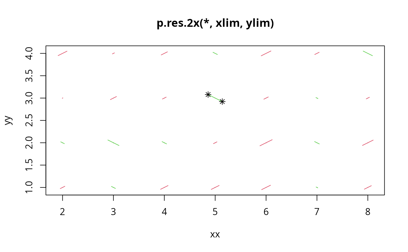
xlab, ylab, main: axis labels, and title see title, each with a sensible default. To suppress, use, e.g., main = "".
xlim, ylim: the basic x- and y- axis extents, see plot.default. Note that these will be slightly extended such that segments are not cut off.
...: further arguments passed to plot, or p.res.2x.default(), respectively.
data: (for the formula method:) a data frame or a fitted "lm" object.

Details

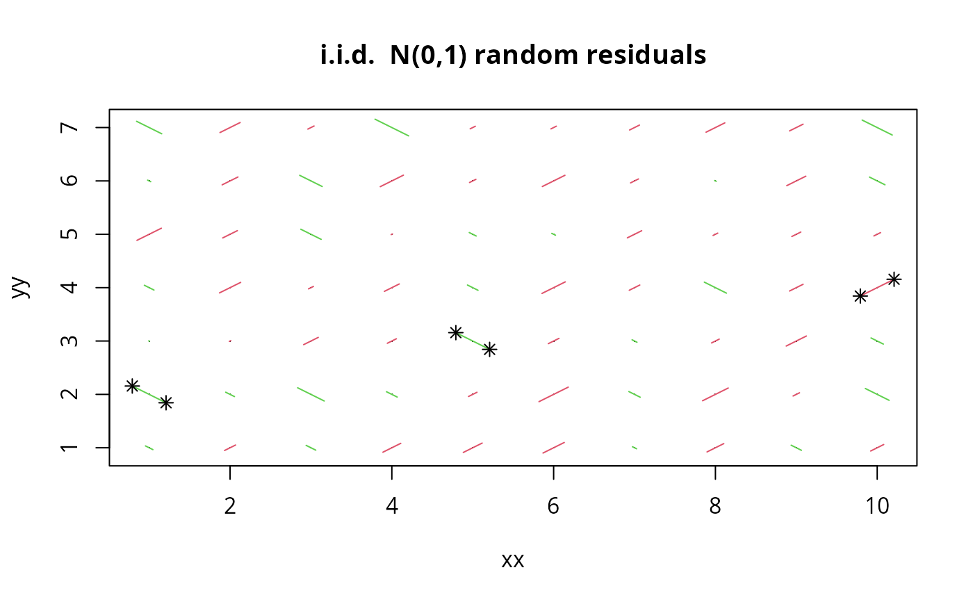
Each residual zz[i] is visualized as line segment centered at \((xx_i,yy_i)\), \(i=1,\dots,n\), where the lengths of the segments are proportional to the absolute values \(\|zz_i\|\).

Positive residuals' line segments have slope \(+1\), and negative ones slope \(-1\), and scol is used to use different colors for negative and positive segments.

The formula interface calls p.res.2fact() when both x and y are factors.

References

Stahel, W.~A. (2008) Statistische Datenanalyse: Eine Einführung für Naturwissenschaftler, 5. Auflage, Vieweg, Wiesbaden; Paragraph 13.8.r and 13.8.v.

Author

Andreas Ruckstuhl in June 1991 and Martin Maechler, in 1992, '94, 2003-4.

Examples

xx <- rep(1:10,7)
yy <- rep(1:7, rep(10,7))
zz <- rnorm(70)
p.res.2x(xx,yy,zz, restricted = 2, main = "i.i.d.  N(0,1) random residuals")


example(lm.influence, echo = FALSE)
#> List of 4
#>  $ hat         : Named num [1:50] 0.0677 0.1204 0.0875 0.0895 0.0696 ...
#>   ..- attr(*, "names")= chr [1:50] "Australia" "Austria" "Belgium" "Bolivia" ...
#>  $ coefficients: num [1:50, 1:5] 0.0916 -0.0747 -0.4752 0.0429 0.6604 ...
#>   ..- attr(*, "dimnames")=List of 2
#>   .. ..$ : chr [1:50] "Australia" "Austria" "Belgium" "Bolivia" ...
#>   .. ..$ : chr [1:5] "(Intercept)" "pop15" "pop75" "dpi" ...
#>  $ sigma       : Named num [1:50] 3.84 3.84 3.83 3.84 3.81 ...
#>   ..- attr(*, "names")= chr [1:50] "Australia" "Austria" "Belgium" "Bolivia" ...
#>  $ wt.res      : Named num [1:50] 0.864 0.616 2.219 -0.698 3.553 ...
#>   ..- attr(*, "names")= chr [1:50] "Australia" "Austria" "Belgium" "Bolivia" ...

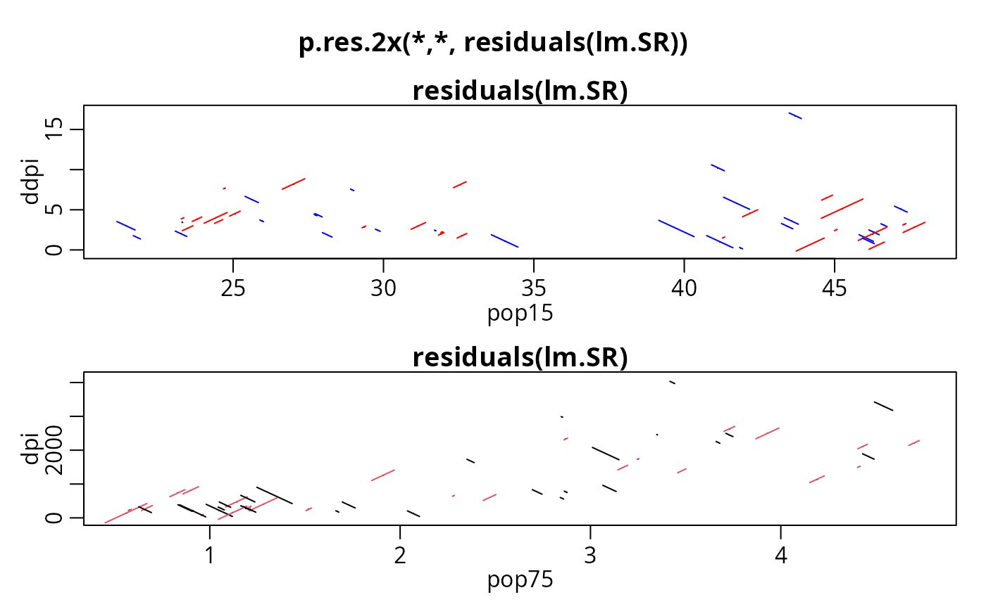
op <- mult.fig(2, marP=c(-1,-1,-1,0), main="p.res.2x(*,*, residuals(lm.SR))")$old.par
with(LifeCycleSavings,
     { p.res.2x(pop15, ddpi, residuals(lm.SR), scol=c("red", "blue"))
       p.res.2x(pop75, dpi,  residuals(lm.SR), scol=2:1)
     })


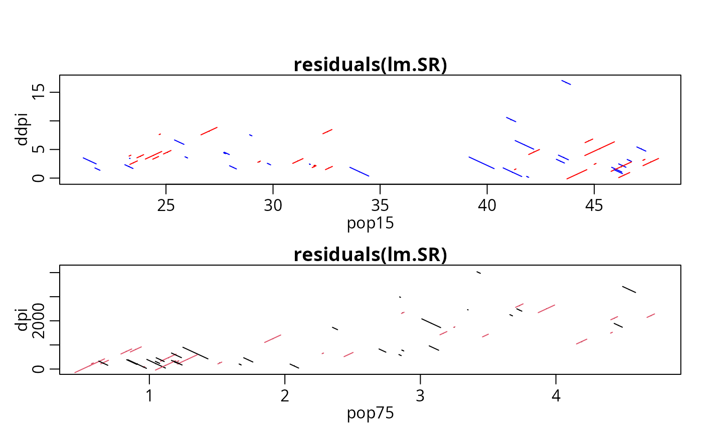
## with formula interface:
p.res.2x(~ pop15 + ddpi, lm.SR, scol=c("red", "blue"))
p.res.2x(~ pop75 +  dpi, lm.SR, scol=2:1)


par(op) # revert par() settings above