Plot scatterplot matrices of parameters, random parameters or covariates

These functions plot scatterplot matrices of parameters, random parameters and covariates.

cov.splom(
  object,
  main = xpose.multiple.plot.title(object = object, plot.text =
    "Scatterplot matrix of covariates", ...),
  varnames = NULL,
  onlyfirst = TRUE,
  smooth = TRUE,
  lmline = NULL,
  ...
)

parm.splom(
  object,
  main = xpose.multiple.plot.title(object = object, plot.text =
    "Scatterplot matrix of parameters", ...),
  varnames = NULL,
  onlyfirst = TRUE,
  smooth = TRUE,
  lmline = NULL,
  ...
)

ranpar.splom(
  object,
  main = xpose.multiple.plot.title(object = object, plot.text =
    "Scatterplot matrix of random parameters", ...),
  varnames = NULL,
  onlyfirst = TRUE,
  smooth = TRUE,
  lmline = NULL,
  ...
)

Arguments

object

An xpose.data object.

main

A string giving the plot title or NULL if none.

varnames

A vector of strings containing labels for the variables in the scatterplot matrix.

onlyfirst

Logical value indicating if only the first row per individual is included in the plot.

smooth

A NULL value indicates that no superposed line should be added to the graph. If TRUE then a smooth of the data will be superimposed.

lmline

logical variable specifying whether a linear regression line should be superimposed over an xyplot. NULL ~ FALSE. (y~x)

...

Other arguments passed to xpose.plot.histogram.

Value

Delivers a scatterplot matrix.

Details

The parameters or covariates in the Xpose data object, as specified in object@Prefs@Xvardef$parms, object@Prefs@Xvardef$ranpar or object@Prefs@Xvardef$covariates, are plotted together as scatterplot matrices.

A wide array of extra options controlling scatterplot matrices are available. See xpose.plot.splom for details.

To control the appearance of the labels and names in the scatterplot matrix plots you can try varname.cex=0.5 and axis.text.cex=0.5 (this changes the tick labels and the variable names to be half as large as normal).

Functions

• cov.splom(): A scatterplot matrix of covariates

• parm.splom(): A scatterplot matrix of parameters

• ranpar.splom(): A scatterplot matrix of random parameters

See also

xpose.plot.splom, xpose.panel.splom, splom, xpose.data-class, xpose.prefs-class

Other specific functions: absval.cwres.vs.cov.bw(), absval.cwres.vs.pred(), absval.cwres.vs.pred.by.cov(), absval.iwres.cwres.vs.ipred.pred(), absval.iwres.vs.cov.bw(), absval.iwres.vs.idv(), absval.iwres.vs.ipred(), absval.iwres.vs.ipred.by.cov(), absval.iwres.vs.pred(), absval.wres.vs.cov.bw(), absval.wres.vs.idv(), absval.wres.vs.pred(), absval.wres.vs.pred.by.cov(), absval_delta_vs_cov_model_comp, addit.gof(), autocorr.cwres(), autocorr.iwres(), autocorr.wres(), basic.gof(), basic.model.comp(), cat.dv.vs.idv.sb(), cat.pc(), cwres.dist.hist(), cwres.dist.qq(), cwres.vs.cov(), cwres.vs.idv(), cwres.vs.idv.bw(), cwres.vs.pred(), cwres.vs.pred.bw(), cwres.wres.vs.idv(), cwres.wres.vs.pred(), dOFV.vs.cov(), dOFV.vs.id(), dOFV1.vs.dOFV2(), data.checkout(), dv.preds.vs.idv(), dv.vs.idv(), dv.vs.ipred(), dv.vs.ipred.by.cov(), dv.vs.ipred.by.idv(), dv.vs.pred(), dv.vs.pred.by.cov(), dv.vs.pred.by.idv(), dv.vs.pred.ipred(), gof(), ind.plots(), ind.plots.cwres.hist(), ind.plots.cwres.qq(), ipred.vs.idv(), iwres.dist.hist(), iwres.dist.qq(), iwres.vs.idv(), kaplan.plot(), par_cov_hist, par_cov_qq, parm.vs.cov(), parm.vs.parm(), pred.vs.idv(), ranpar.vs.cov(), runsum(), wres.dist.hist(), wres.dist.qq(), wres.vs.idv(), wres.vs.idv.bw(), wres.vs.pred(), wres.vs.pred.bw(), xpose.VPC(), xpose.VPC.both(), xpose.VPC.categorical(), xpose4-package

Author

Andrew Hooker & Justin Wilkins

Examples

## Here we load the example xpose database 
xpdb <- simpraz.xpdb

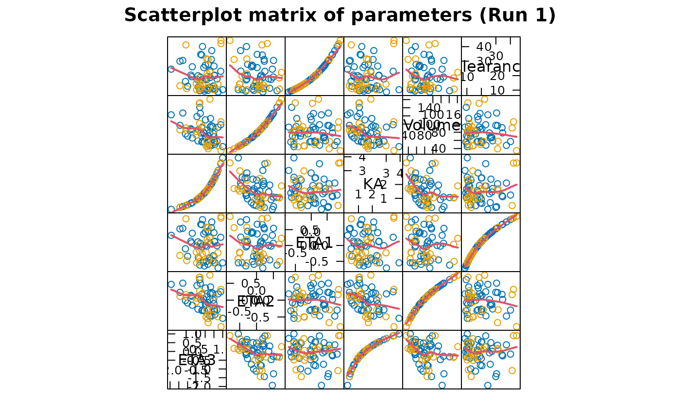
## A scatterplot matrix of parameters, grouped by sex
parm.splom(xpdb, groups="SEX")


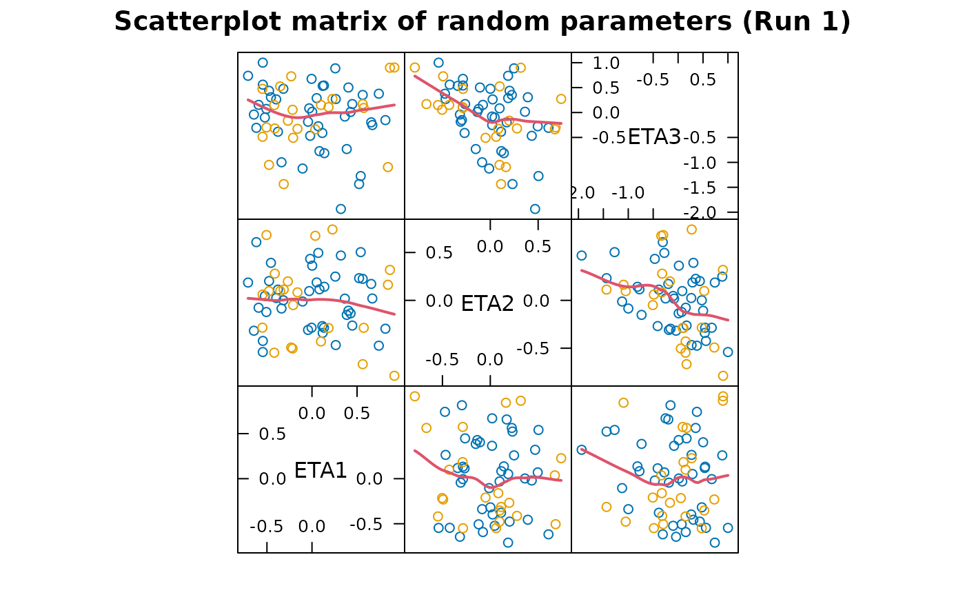
## A scatterplot matrix of ETAs, grouped by sex
ranpar.splom(xpdb, groups="SEX")


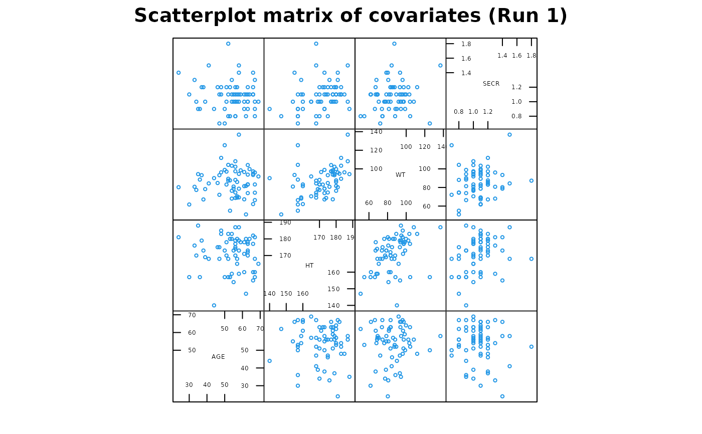
## Covariate scatterplots, with text customization
cov.splom(xpdb, varname.cex=0.4, axis.text.cex=0.4, smooth=NULL, cex=0.4)
#> SEX is categorical and will not be
#>  shown in the scatterplot
#> RACE is categorical and will not be
#>  shown in the scatterplot
#> SMOK is categorical and will not be
#>  shown in the scatterplot
#> HCTZ is categorical and will not be
#>  shown in the scatterplot
#> PROP is categorical and will not be
#>  shown in the scatterplot
#> CON is categorical and will not be
#>  shown in the scatterplot
#> OCC is categorical and will not be
#>  shown in the scatterplot