Diagnostic Displays

Kyle Baron

2026-07-01

Overview

This feature set provides standardized displays of diagnostics, including

• ETA versus covariates
• NPDE or CWRES versus covariates
• NPDE or CWRES diagnostics as
  • single, comprehensive panel
  • just scatter plots
  • just histogram and QQ plots

In addition to these standard displays, the user can get an object back containing the component plots for the standardized displays that you can arrange yourself.

library(pmplots)
data <- pmplots_data_obs()
id <- pmplots_data_id()
cont <- c("WT//Weight (kg)", "AGE//Age (years)")
cat <- c("CPc//Child-Pugh", "STUDYc//Study")
covs <- c(cont,cat)
etas <- c("ETA1//ETA-CL", "ETA2//ETA-V", "ETA3//ETA-KA")

ETA versus covariates

The basic / default behavior is to get a list of arranged plots, one for each ETA

p <- eta_covariate(id, x = covs, y = etas)

names(p) 

## [1] "ETA1" "ETA2" "ETA3"

p$ETA1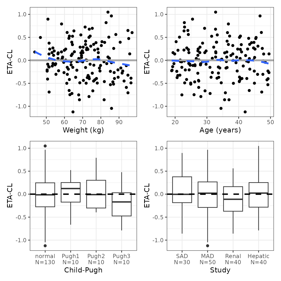

We can label the panels; thinking about making this the default

p <- eta_covariate(id, x = covs, y = etas, tag_levels = "A")

p$ETA1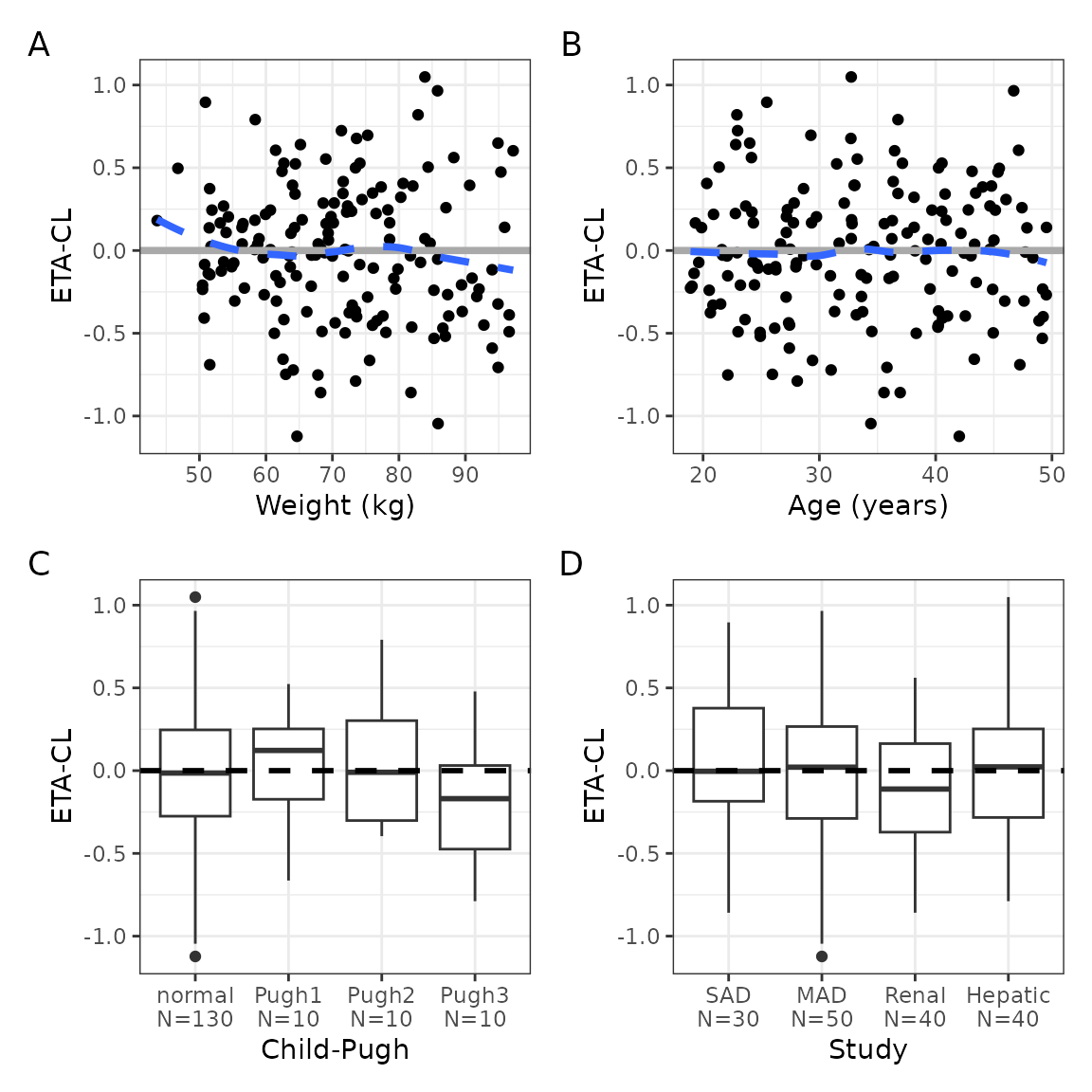

We can arrange this by column instead

p <- eta_covariate(id, x = covs, y = etas, tag_levels = "A", byrow = FALSE)

p$ETA1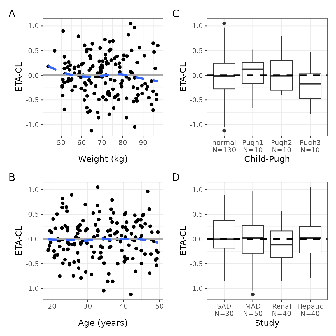

Or we can group by the covariate rather than the ETA using the transpose argument

p <- eta_covariate(id, x = covs, y = etas, tag_levels = "A", transpose = TRUE)

names(p)

## [1] "WT"     "AGE"    "CPc"    "STUDYc"

Now, we have all the ETAs for each covariate on the same page

p$AGE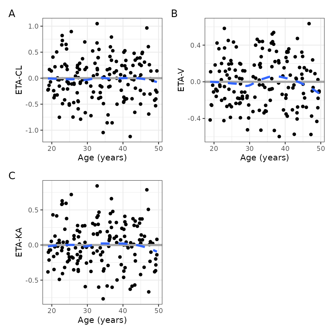

and

p$CPc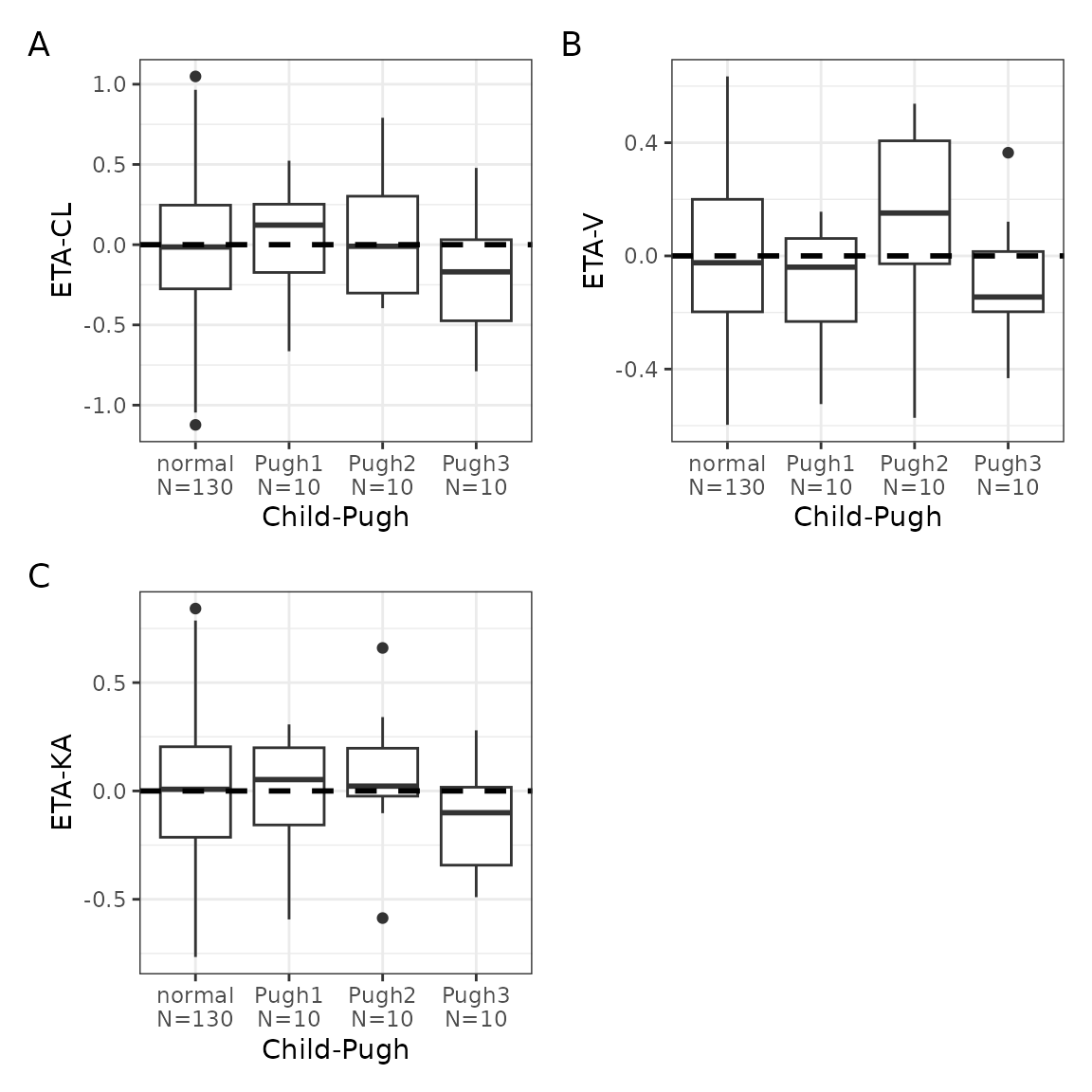

We can make a custom arrangement using the patchwork arrangement operators

p <- eta_covariate_list(id, x = covs, y = etas)

with(p$ETA1, (WT / (CPc + STUDYc) / AGE), tag_levels = "A")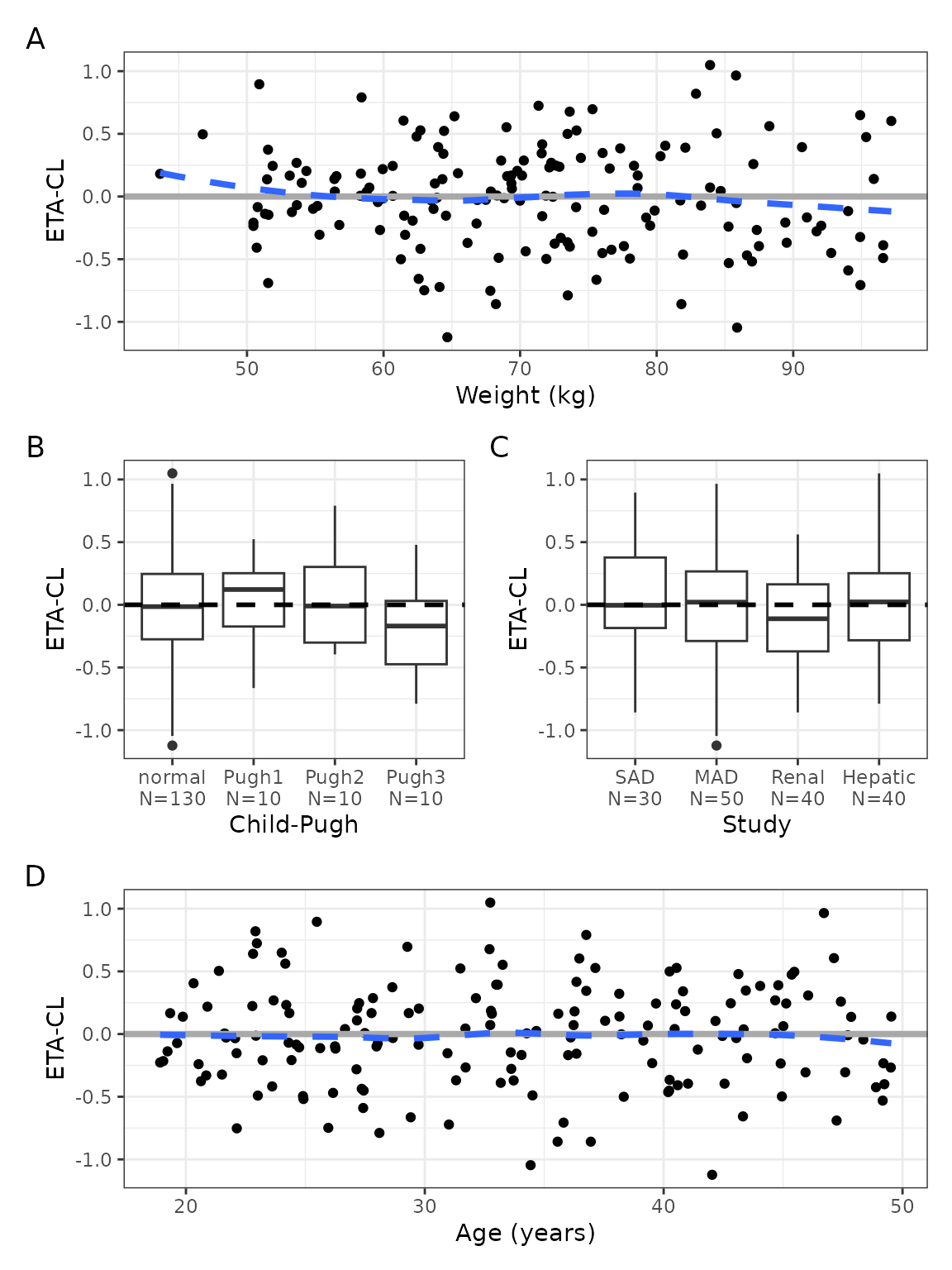

Standard NPDE diagnostics

You can get all the NPDE diagnostics in a single graphic. This might be too much for a report, but could be handy for your model checkout script

npde_panel(data, tag_levels = "A")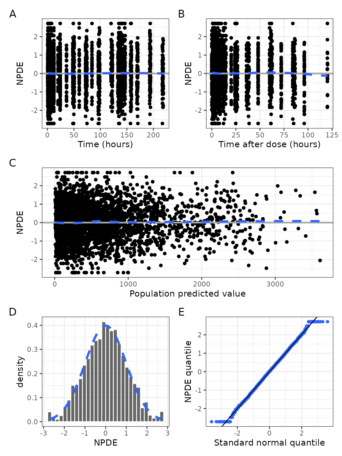

or just the histogram and qq plot

npde_hist_q(data, tag_levels = "A")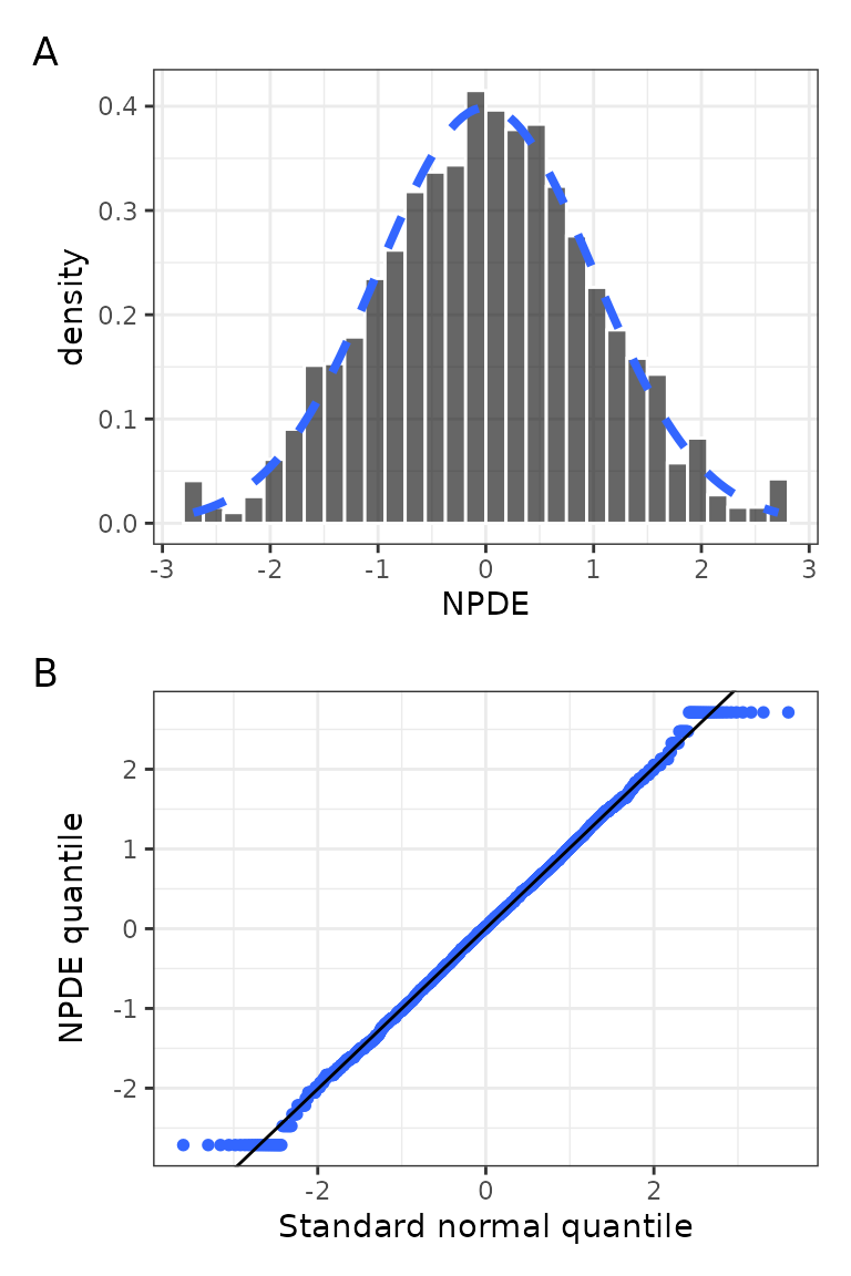

or just the scatter plots in long format

npde_scatter(data, tag_levels = "A")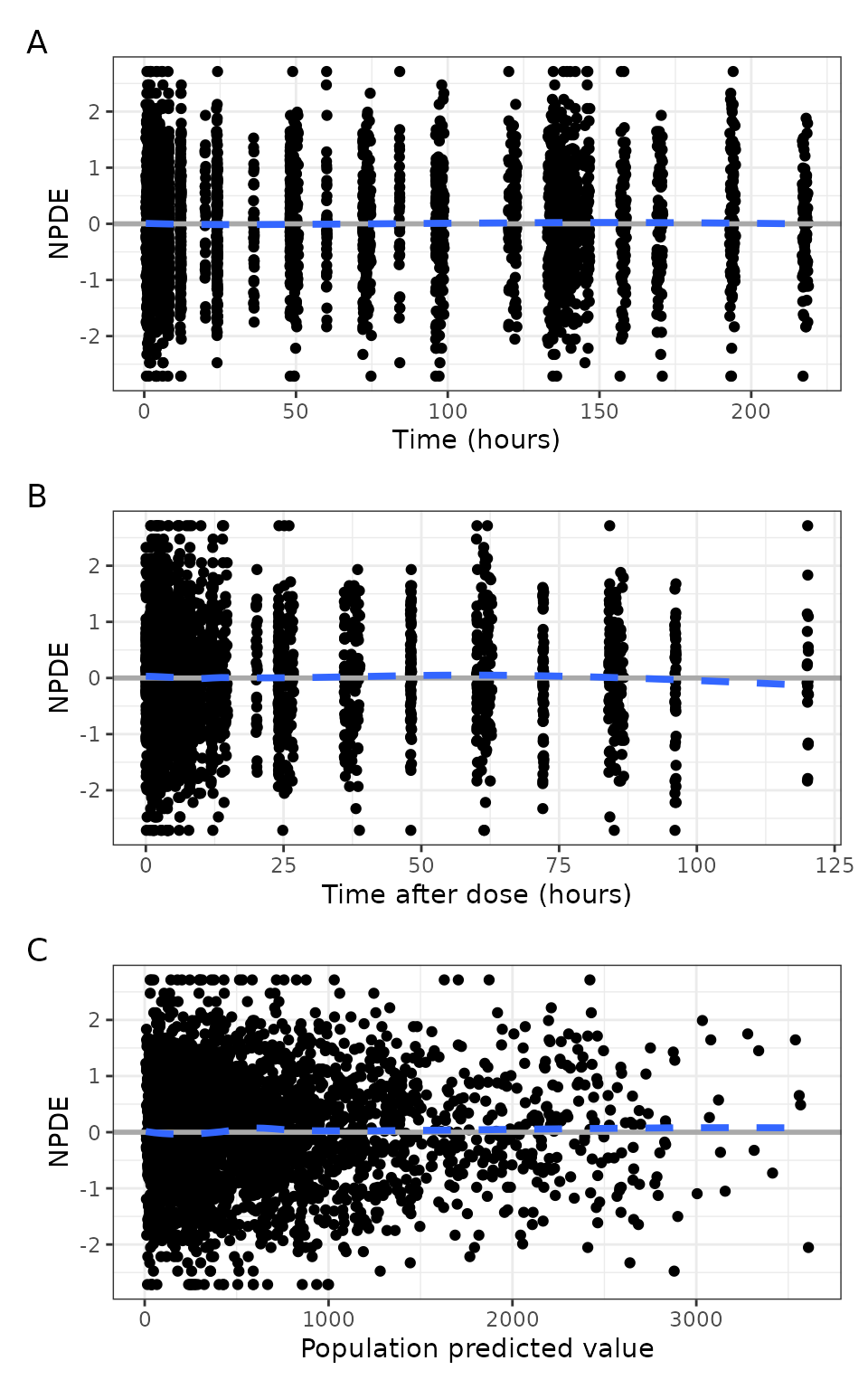

or compact format

npde_scatter(data, tag_levels = "A", compact = TRUE)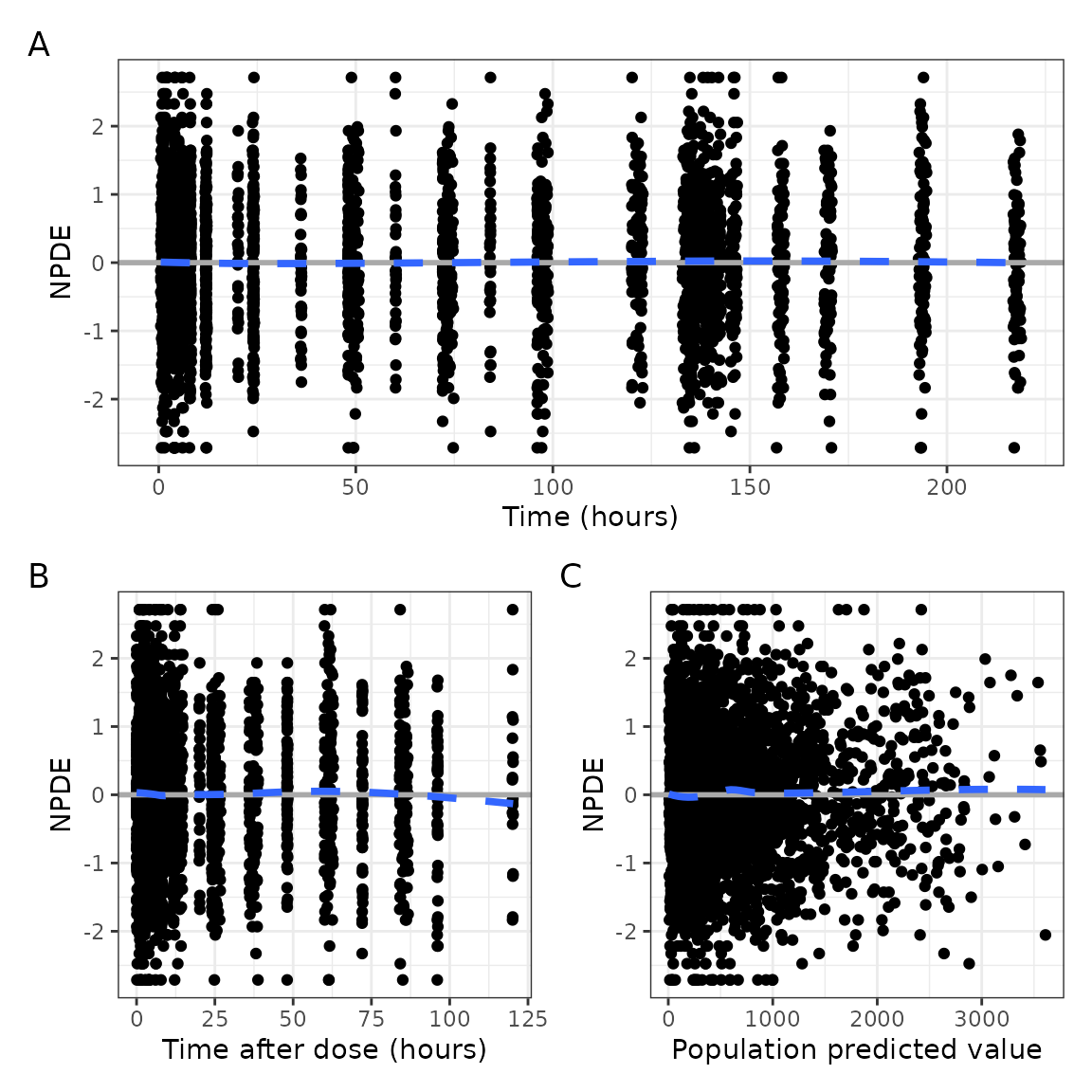

You can also customize the layout to be whatever you want

plots <- npde_panel_list(data)

with(plots, time / (hist + q + tad), tag_levels = "A")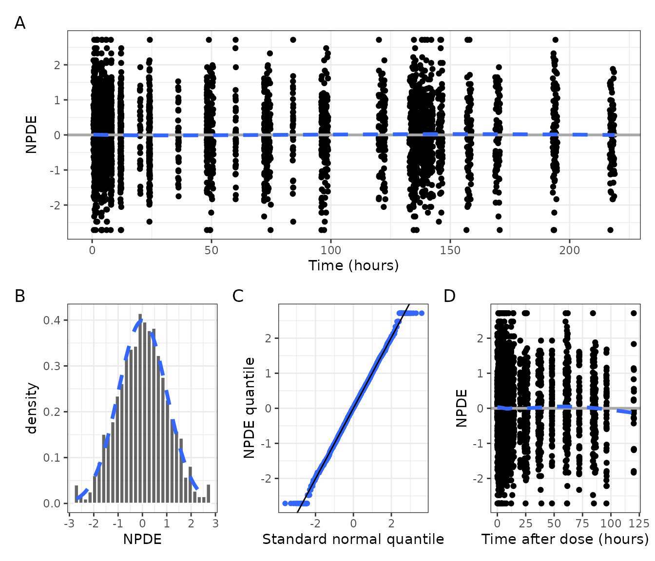 

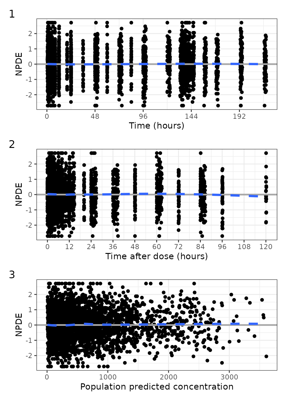
There is some customization for the plot axes and titles, including

• x-axis tick intervals for time and tad
• x-axis units for time and tad
• the name for pred

npde_scatter(
  data, 
  xby_tad = 12, 
  xby_time = 48,
  xname = "concentration", 
  tag_levels = 1
)

NPDE versus covariates

This works like eta_covariate()

npde_covariate(data, covs, tag_levels = "a", byrow = FALSE)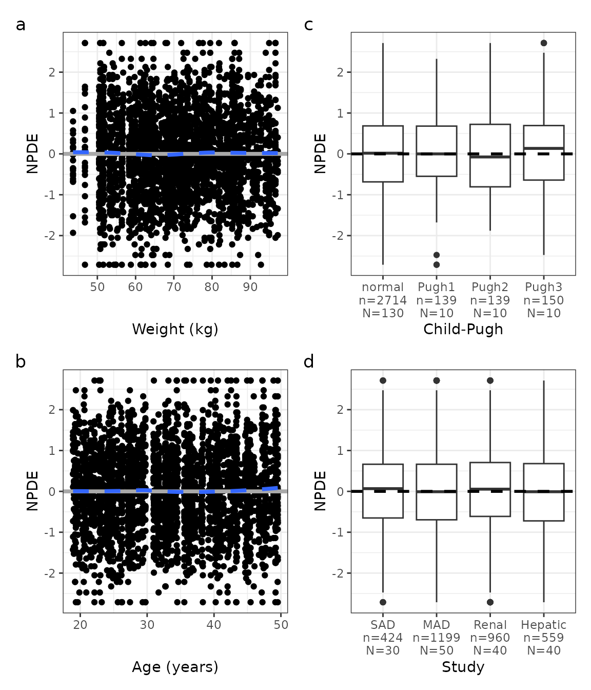

plots <- npde_covariate_list(data, covs)

names(plots)

## [1] "WT"     "AGE"    "CPc"    "STUDYc"

with(plots, (AGE + WT) / CPc / STUDYc, tag_levels = "i")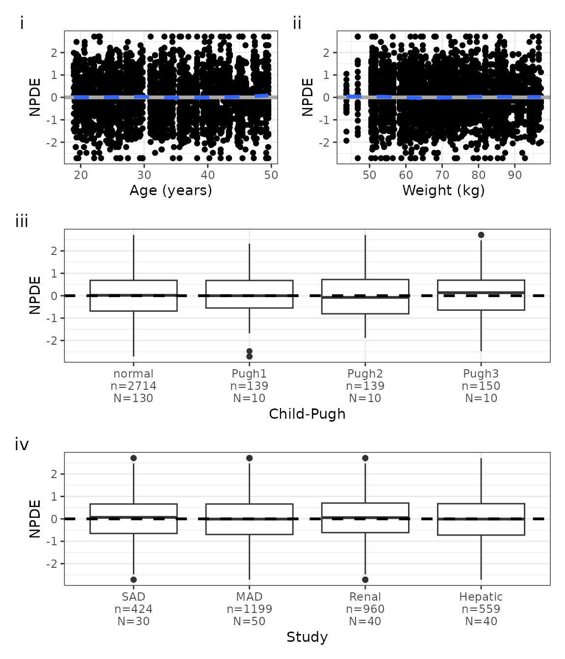

Standard CWRES diagnostics

The behavior / feature set looks just like the NPDE plots for both standard diagnostics and covariates.

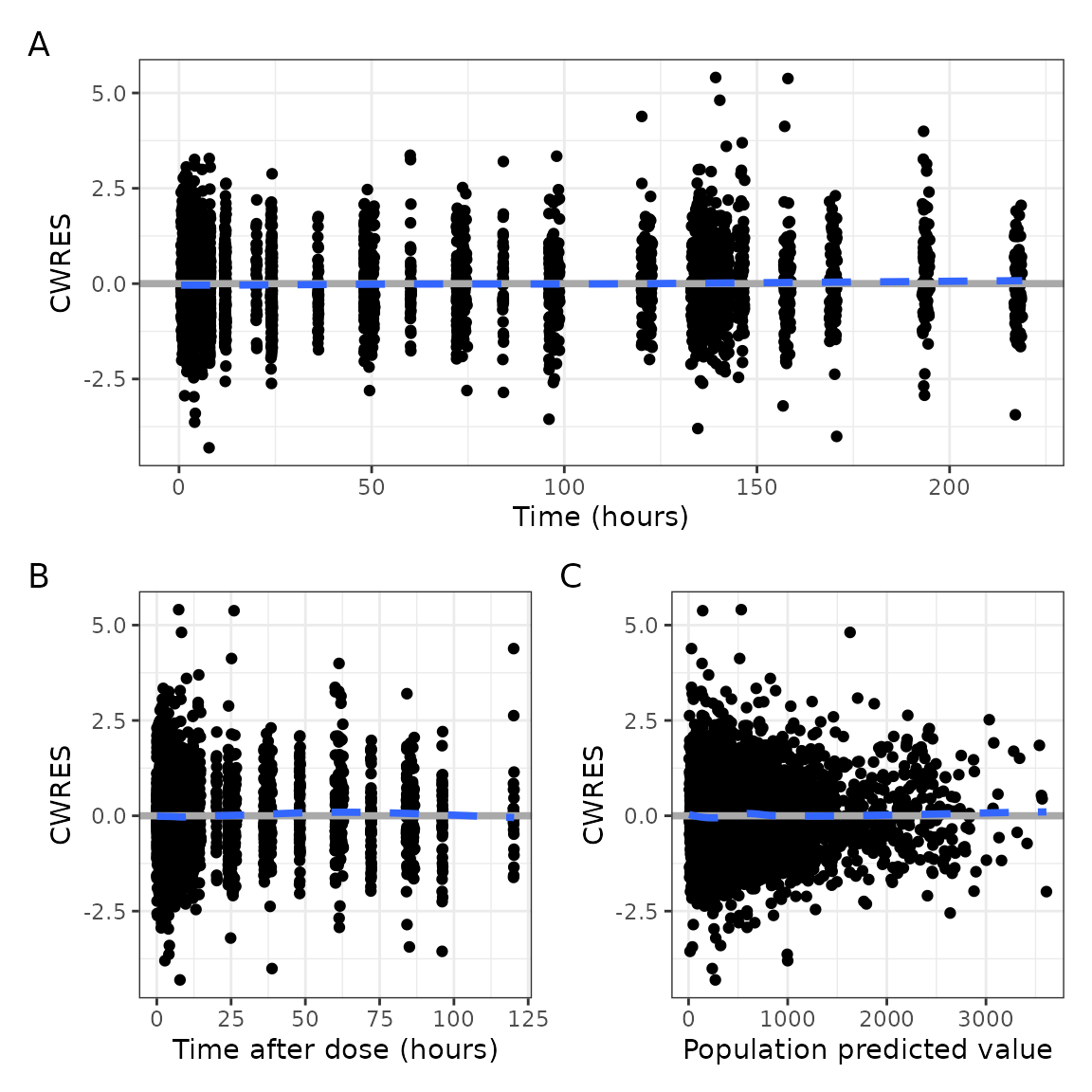
cwres_scatter(data, tag_levels = "A", compact = TRUE)