Skip to contents

The purpose of this vignette is to display all high-level plots available in GGally to be used in particular with ggduo() and ggpairs(). The name of all the corresponding functions are of the form ggally_*(). Most of them accept a discrete variables to be passed to the colour aesthetic.

We can distinct bivariate plots requiring two variables for x and y axis respectively and diagonal plots when the same variable is plotted on x and y axis.

library(GGally, quietly = TRUE)
data(tips)

Bivariate plots

with 2x continuous variables

ggally_autopoint()

ggally_autopoint(tips, aes(x = total_bill, y = tip))
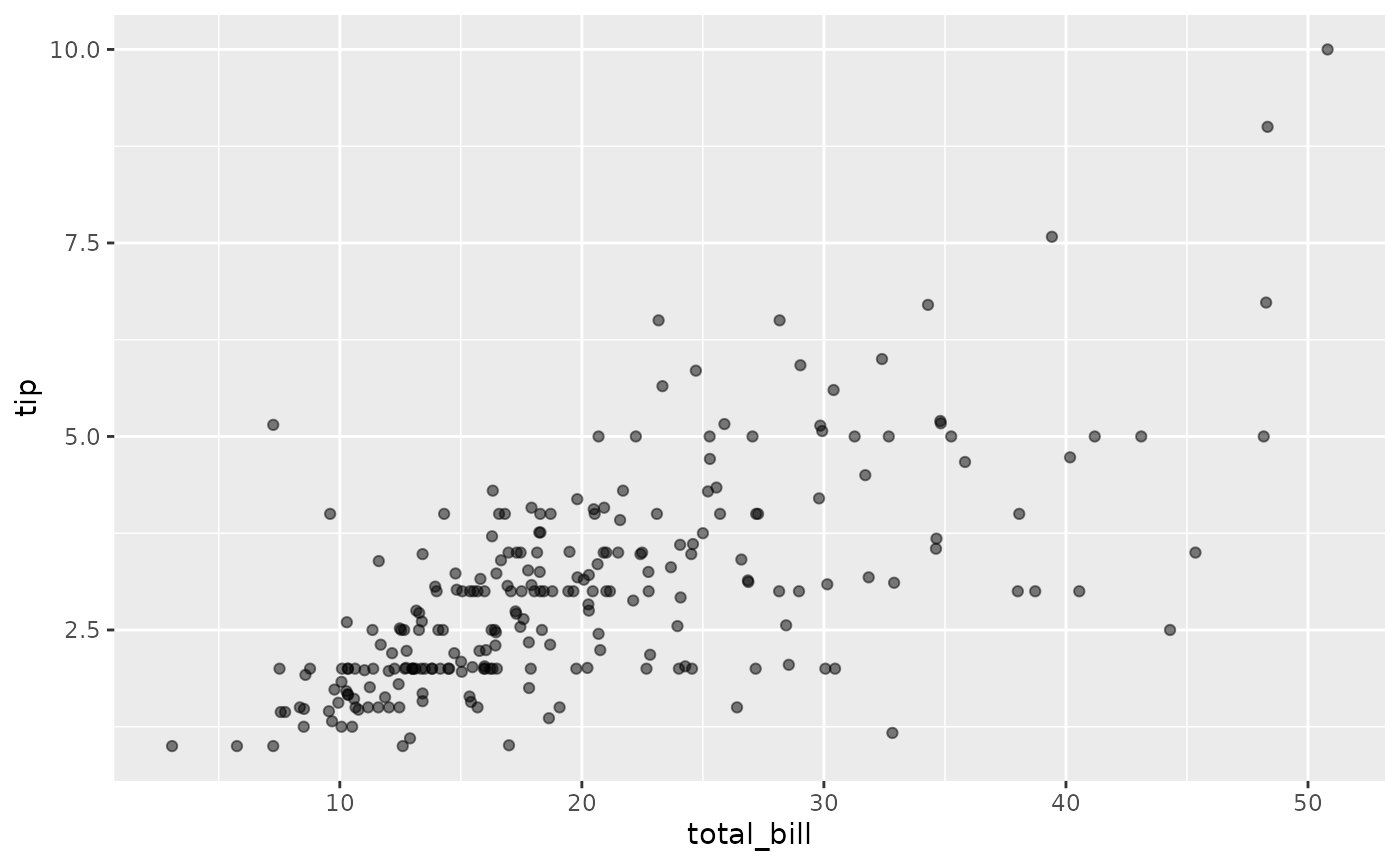
Scatterplot of tip versus total bill. Tips rise with the bill.

ggally_autopoint(tips, aes(x = total_bill, y = tip, colour = time))
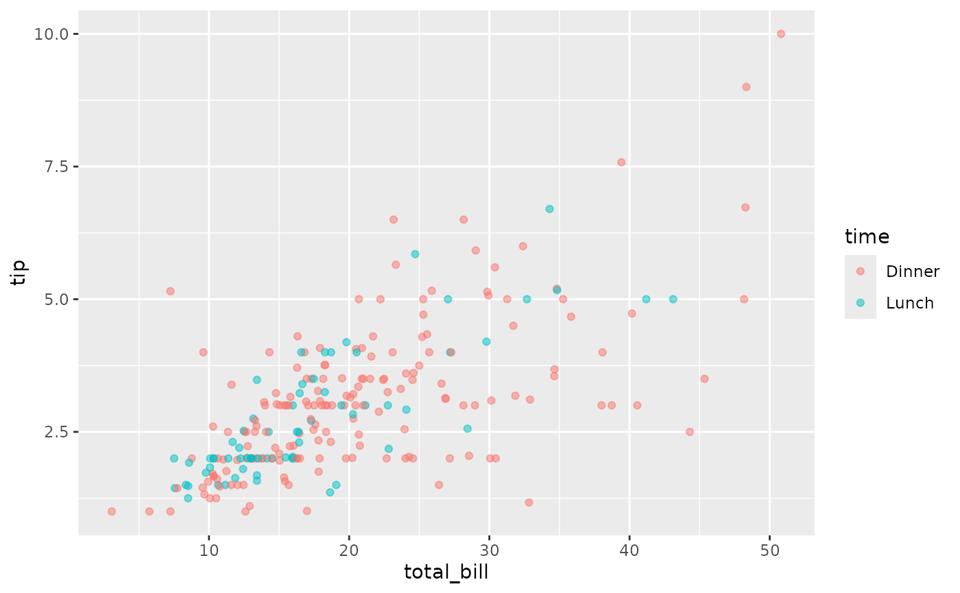
Scatterplot of tip versus total bill, coloured by time (dinner or lunch). Tips rise with the bill at both meals.

ggally_cor()

ggally_cor(tips, aes(x = total_bill, y = tip))
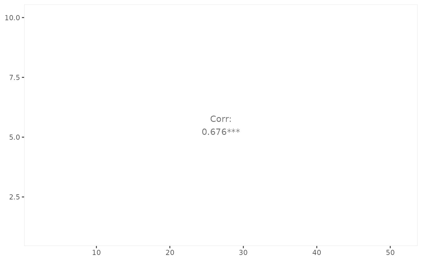
Text panel showing the correlation between total bill and tip: Corr 0.676 with three significance stars.

ggally_cor(tips, aes(x = total_bill, y = tip, colour = time))
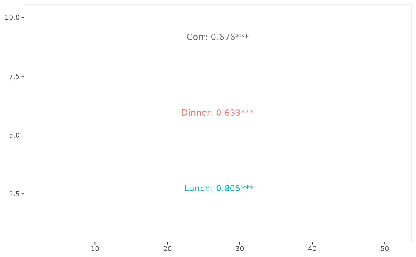
Text panel showing the overall correlation between total bill and tip (0.676), then the dinner (0.633) and lunch (0.805) correlations in their own colours.

See also ggally_statistic().

ggally_density()

ggally_density(tips, aes(x = total_bill, y = tip))
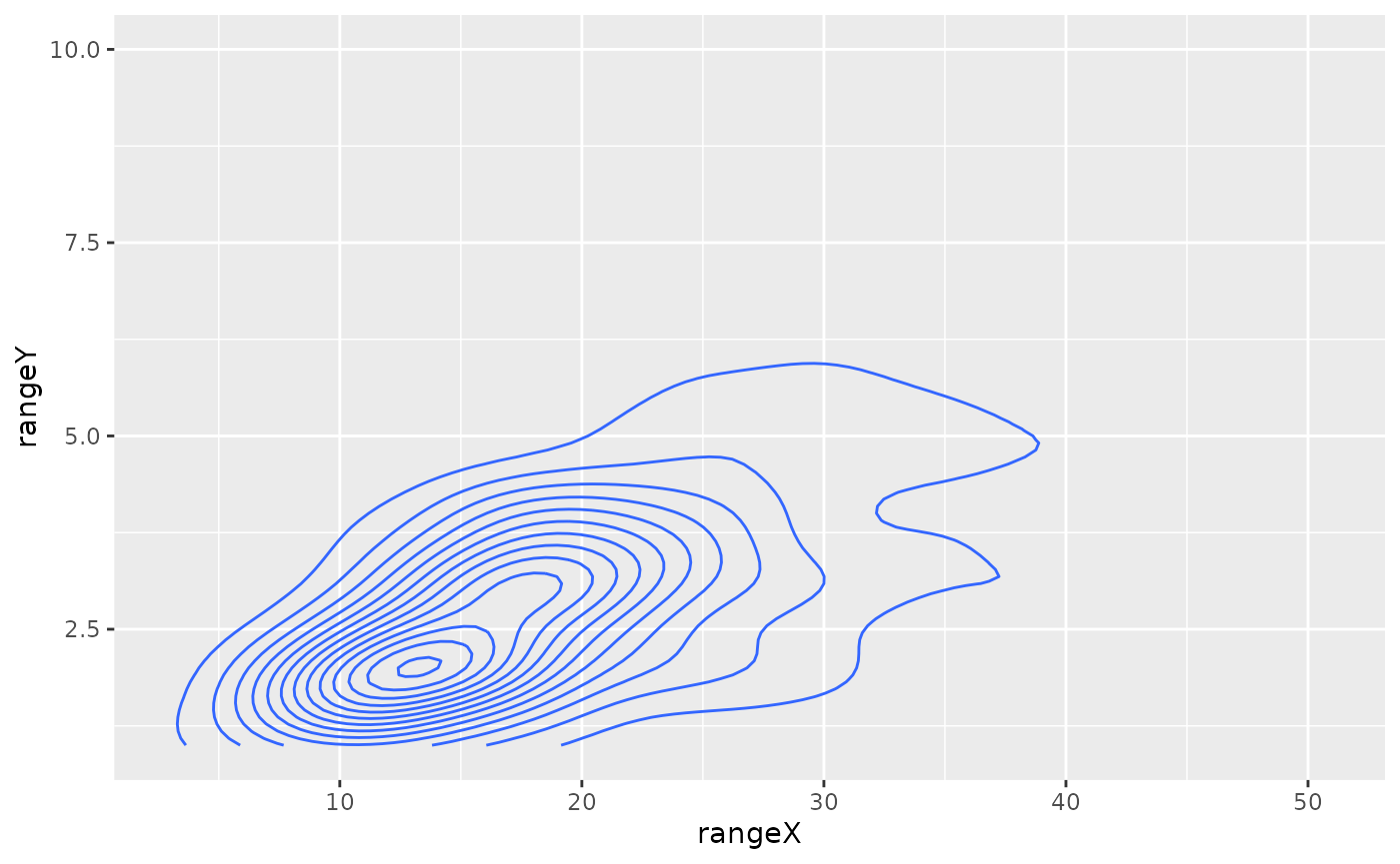
2D density contour plot of tip versus total bill. Most bills sit near 15 dollars with tips near 2 dollars.

ggally_density(tips, aes(x = total_bill, y = tip, colour = time))
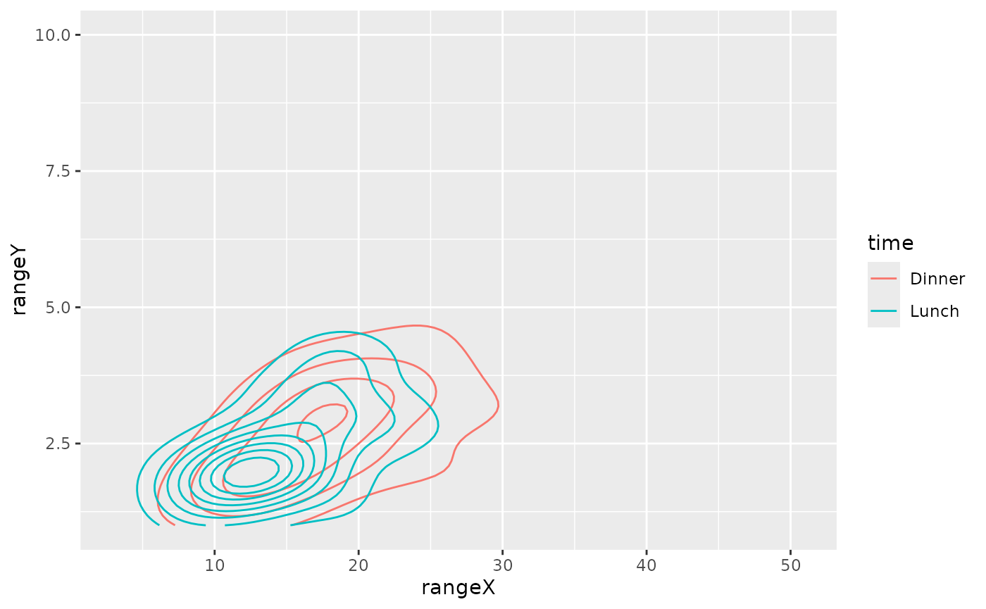
2D density contour plot of tip versus total bill, with separate contours coloured by time. Lunch contours sit at slightly lower bills than dinner.

ggally_points()

ggally_points(tips, aes(x = total_bill, y = tip))
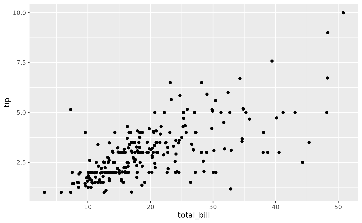
Scatterplot of tip versus total bill. Tips rise with the bill.

ggally_points(tips, aes(x = total_bill, y = tip, colour = time))
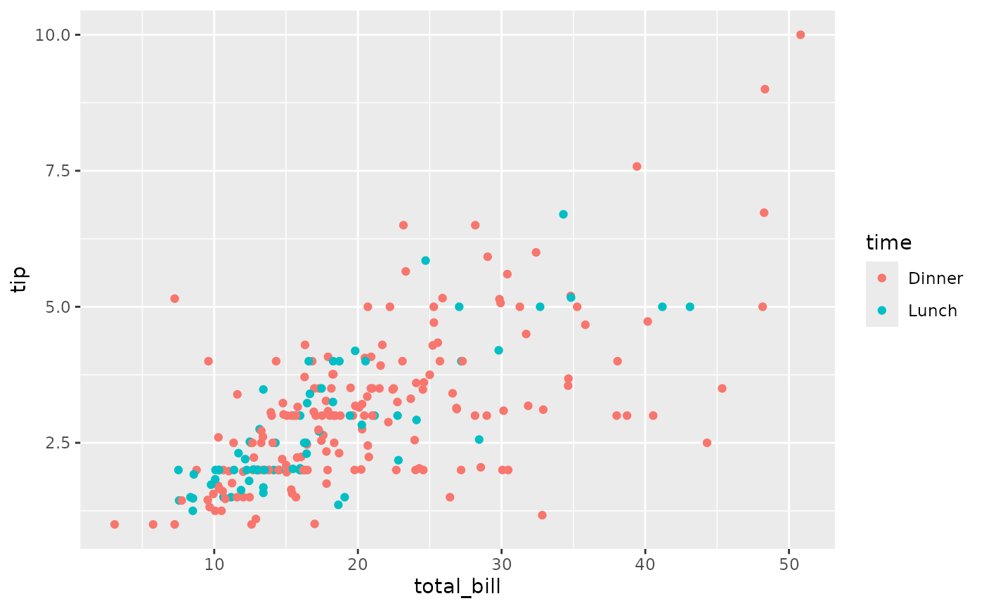
Scatterplot of tip versus total bill, coloured by time. Tips rise with the bill at both meals.

ggally_smooth(), ggally_smooth_lm() & ggally_smooth_loess()

ggally_smooth_lm(tips, aes(x = total_bill, y = tip))
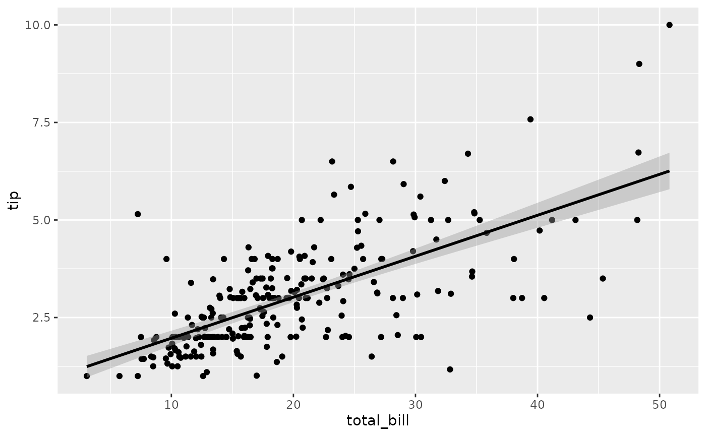
Scatterplot of tip versus total bill with a straight linear fit and confidence band. The line slopes upward.

ggally_smooth_lm(tips, aes(x = total_bill, y = tip, colour = time))
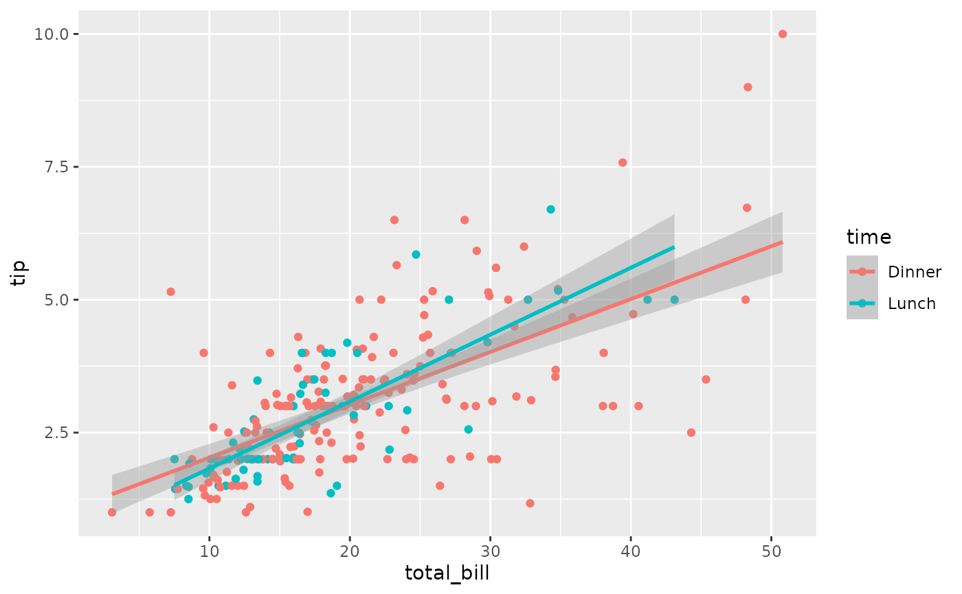
Scatterplot of tip versus total bill coloured by time, with a separate linear fit for dinner and lunch. Both lines slope upward.


ggally_smooth_loess(tips, aes(x = total_bill, y = tip))
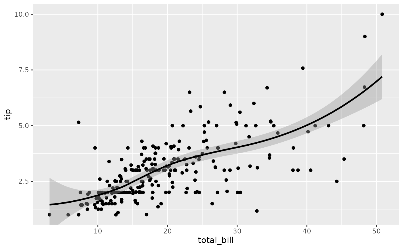
Scatterplot of tip versus total bill with a curved loess fit and confidence band. The curve rises with the bill.

ggally_smooth_loess(tips, aes(x = total_bill, y = tip, colour = time))
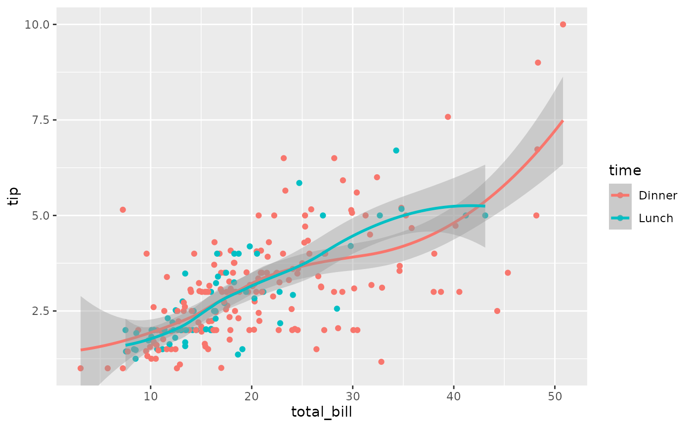
Scatterplot of tip versus total bill coloured by time, with a separate loess curve for dinner and lunch. Both curves rise with the bill.

See also ggally_smooth() for more options.

with 2x discrete variables

ggally_colbar()

ggally_colbar(tips, aes(x = day, y = smoker))
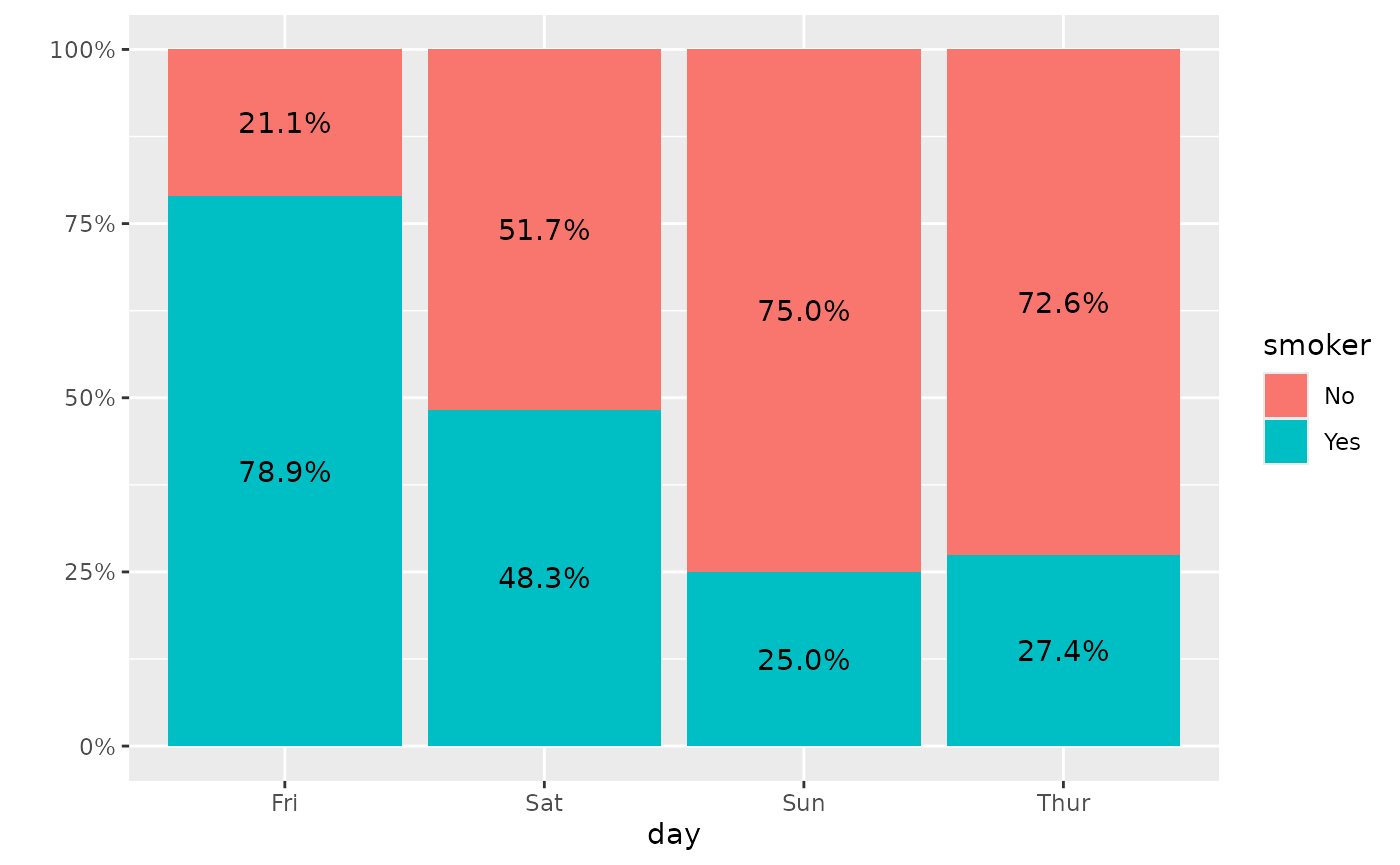
Stacked bar chart of the percentage of smokers and non-smokers within each day, with percent labels. Friday has the most smokers (79 percent); Sunday and Thursday have the fewest.

Note: the colour aesthetic is not taken into account.

ggally_autopoint()

ggally_autopoint(tips, aes(x = day, y = smoker))
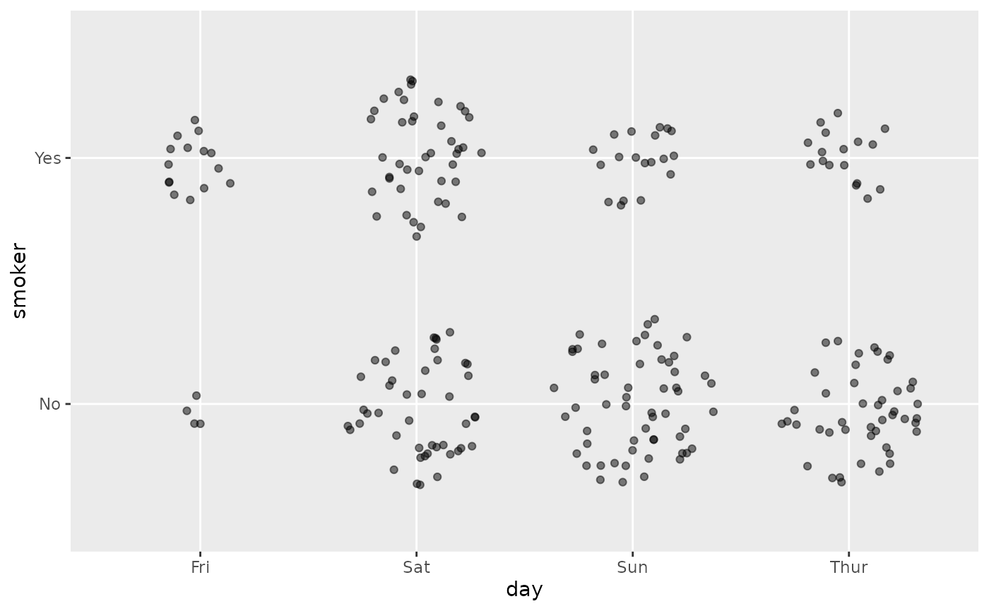
Jittered point plot of smoker versus day. Each point is one bill, and the clouds show how many bills fall in each day and smoker pair.

ggally_autopoint(tips, aes(x = day, y = smoker, colour = time))
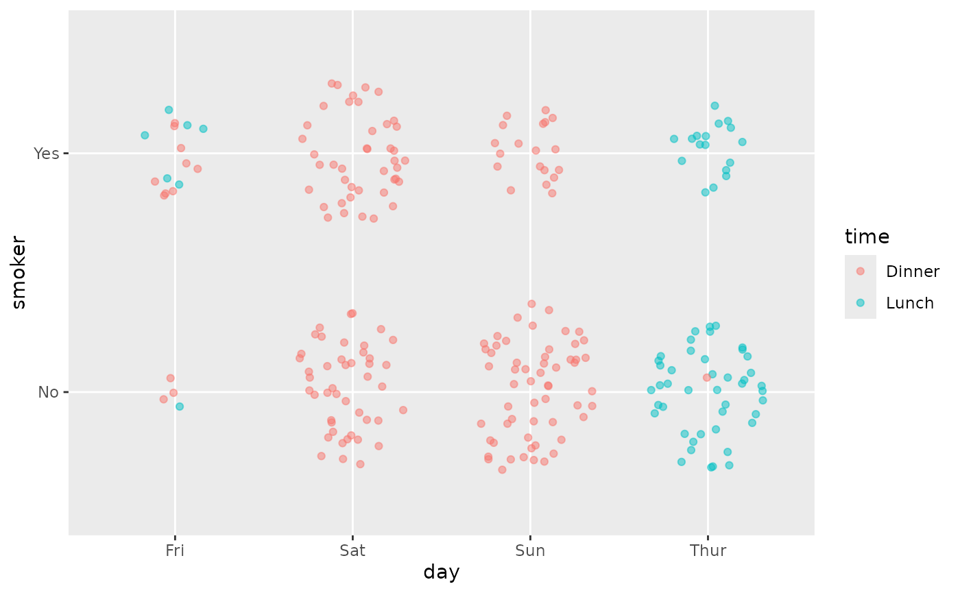
Jittered point plot of smoker versus day, coloured by time. Thursday is almost all lunch, while Saturday and Sunday are all dinner.

ggally_count()

ggally_count(tips, aes(x = day, y = smoker))
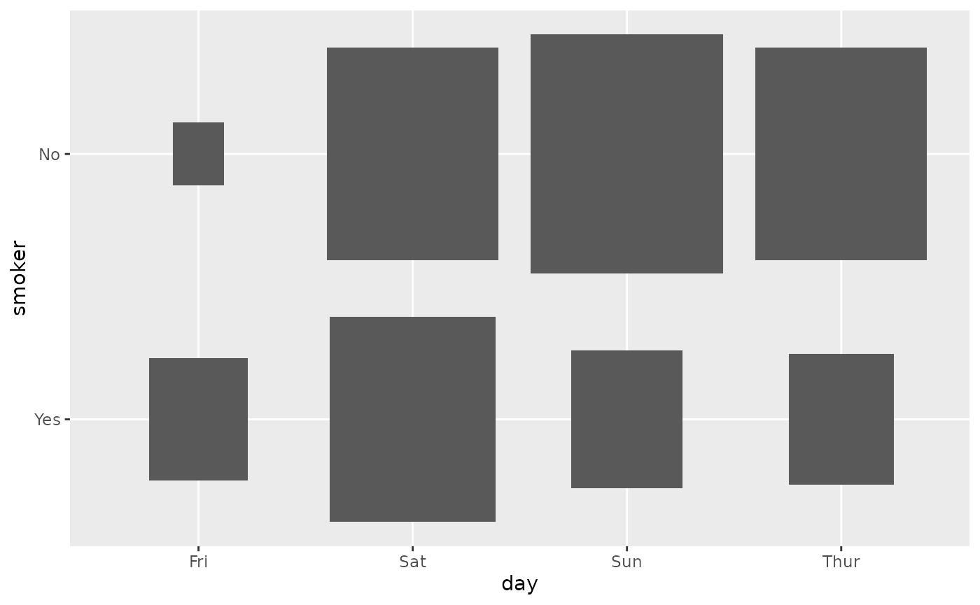
Grid of grey rectangles for smoker versus day, sized by the number of bills. Friday non-smokers is the smallest cell.

ggally_count(tips, aes(x = day, y = smoker, colour = time))
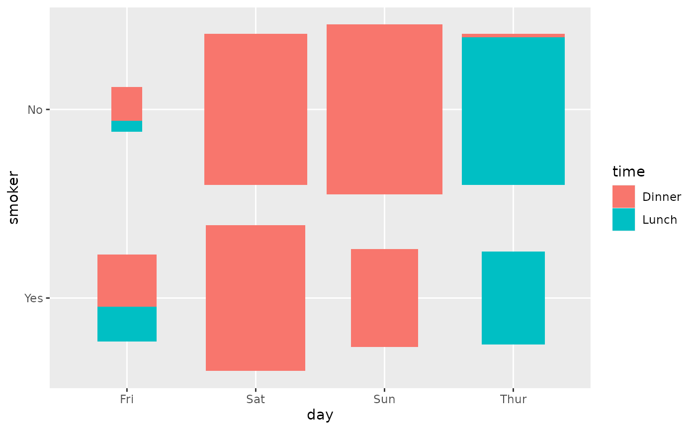
Grid of rectangles for smoker versus day, sized by the number of bills and filled by time. Thursday is mostly lunch and the weekend is all dinner.

ggally_cross()

ggally_cross(tips, aes(x = day, y = smoker))
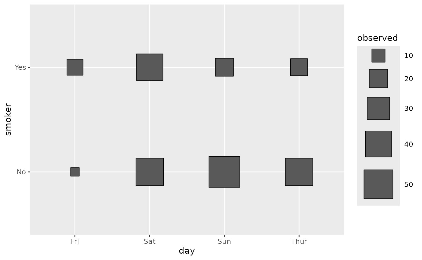
Cross plot of smoker versus day with squares sized by the observed count. Friday non-smokers is the smallest square.

ggally_cross(tips, aes(x = day, y = smoker, colour = time))
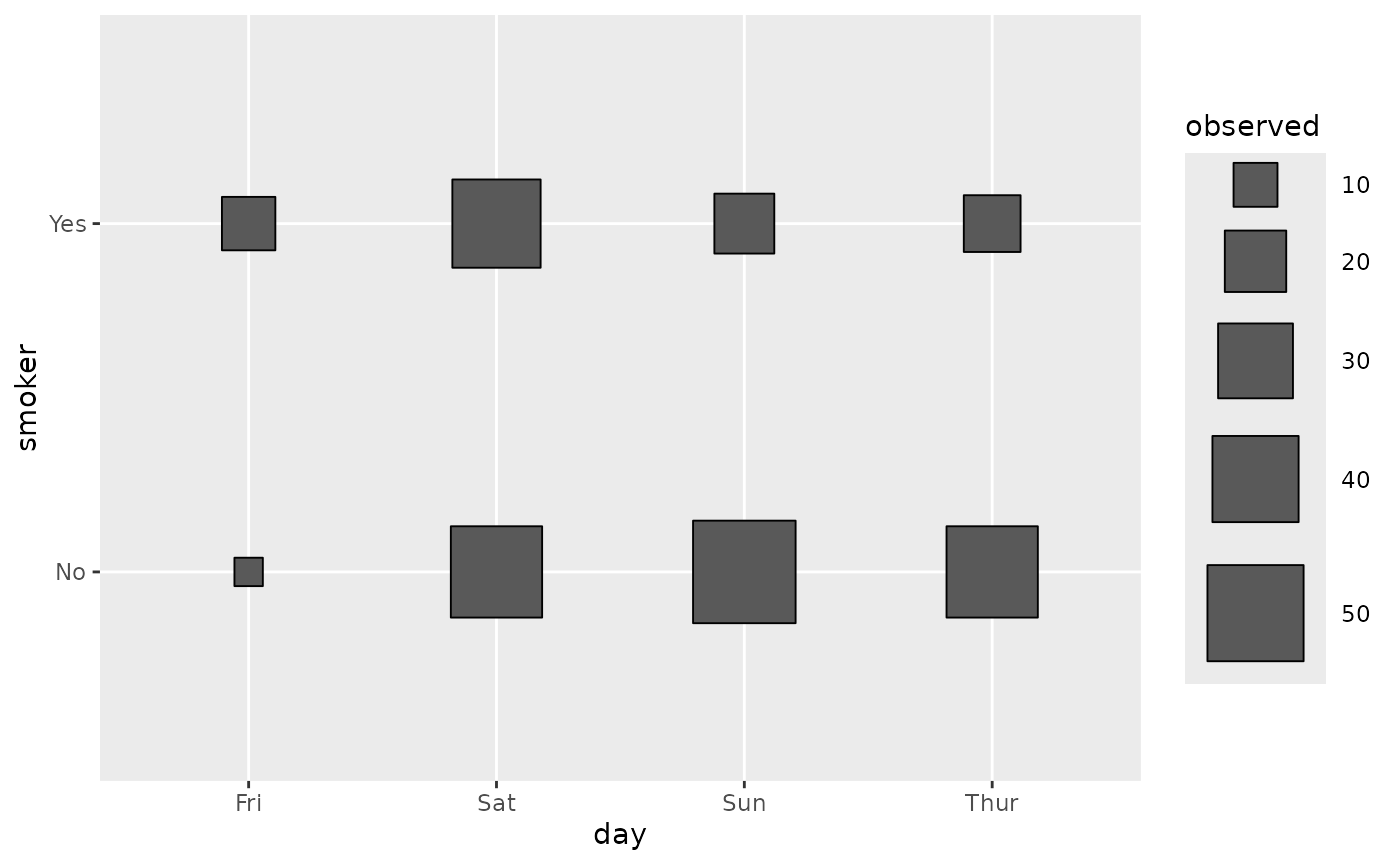
The same cross plot of smoker versus day; colouring by time is ignored, so it looks identical to the first.

ggally_cross(tips, aes(x = day, y = smoker, colour = smoker))
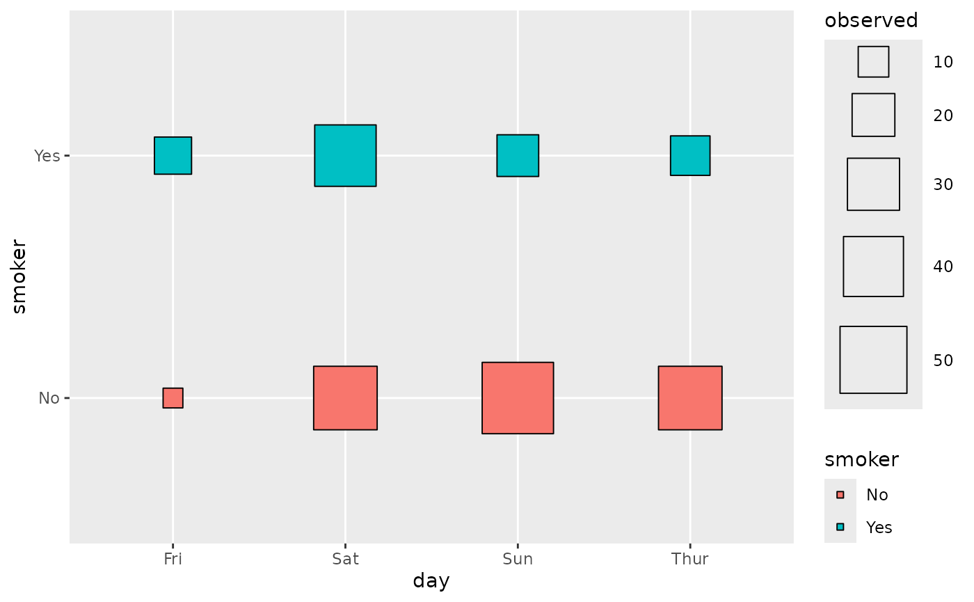
Cross plot of smoker versus day with squares sized by count and coloured by smoker.

Note: colour aesthetic is taken into account only if it corresponds to x or to y.

ggally_crosstable()

ggally_crosstable(tips, aes(x = day, y = smoker))
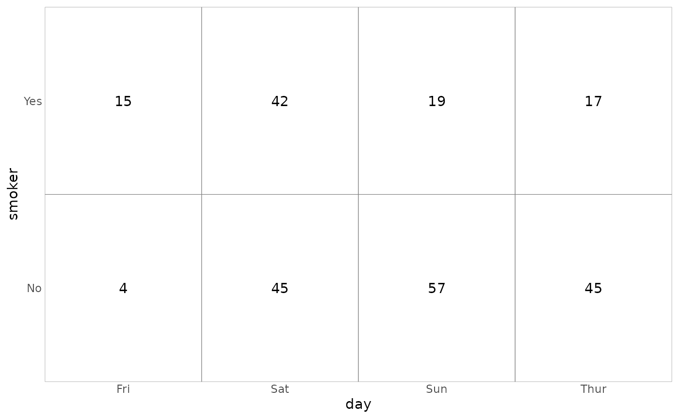
Table of counts of smoker versus day, with one number per cell. Sunday non-smokers is the largest count (57) and Friday non-smokers the smallest (4).

ggally_crosstable(tips, aes(x = day, y = smoker), cells = "col.prop", fill = "std.resid")
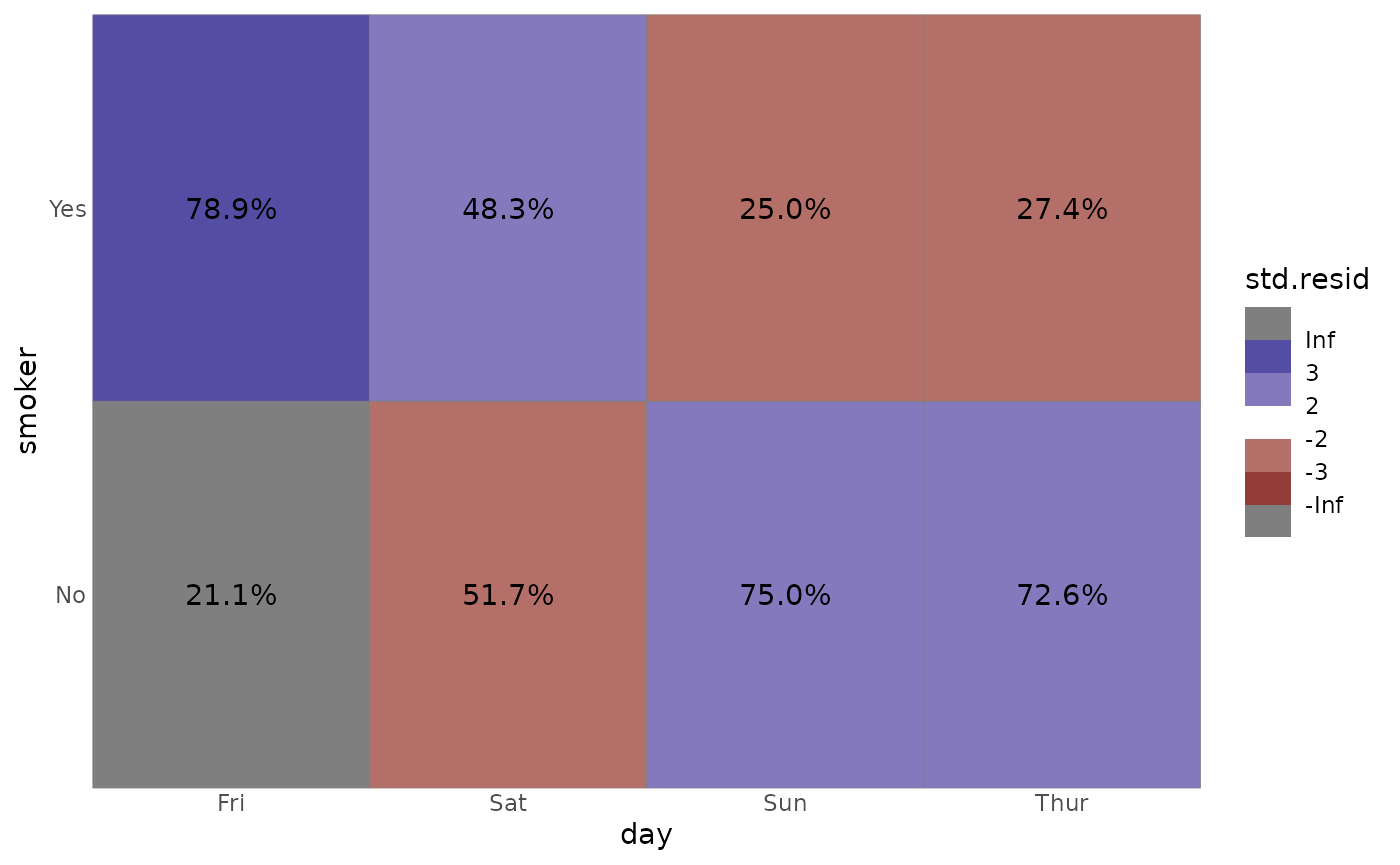
Table of column percentages of smoker versus day, with cells filled by standardized residuals. Friday smokers are much more common than expected; Sunday and Thursday smokers are less common.

Note: colour aesthetic is not taken into account.

ggally_facetbar()

ggally_facetbar(tips, aes(x = day, y = smoker))
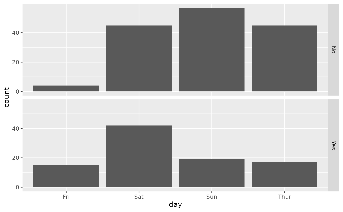
Bar charts of bill counts by day, in one facet per smoker status. Non-smokers peak on Sunday; smokers peak on Saturday.

ggally_facetbar(tips, aes(x = day, y = smoker, colour = time))
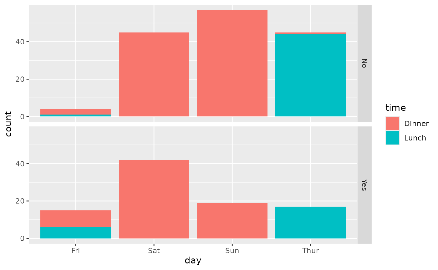
Bar charts of bill counts by day in one facet per smoker status, with bars stacked by time. Thursday bars are almost all lunch and weekend bars are all dinner.

ggally_ratio()

ggally_ratio(tips, aes(x = day, y = smoker))
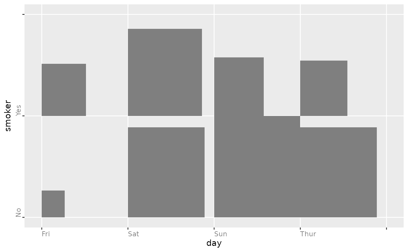
Mosaic plot of smoker versus day where each rectangle's area shows the number of bills. Saturday and Sunday have the largest areas.

ggally_ratio(tips, aes(x = day, y = smoker, colour = time))
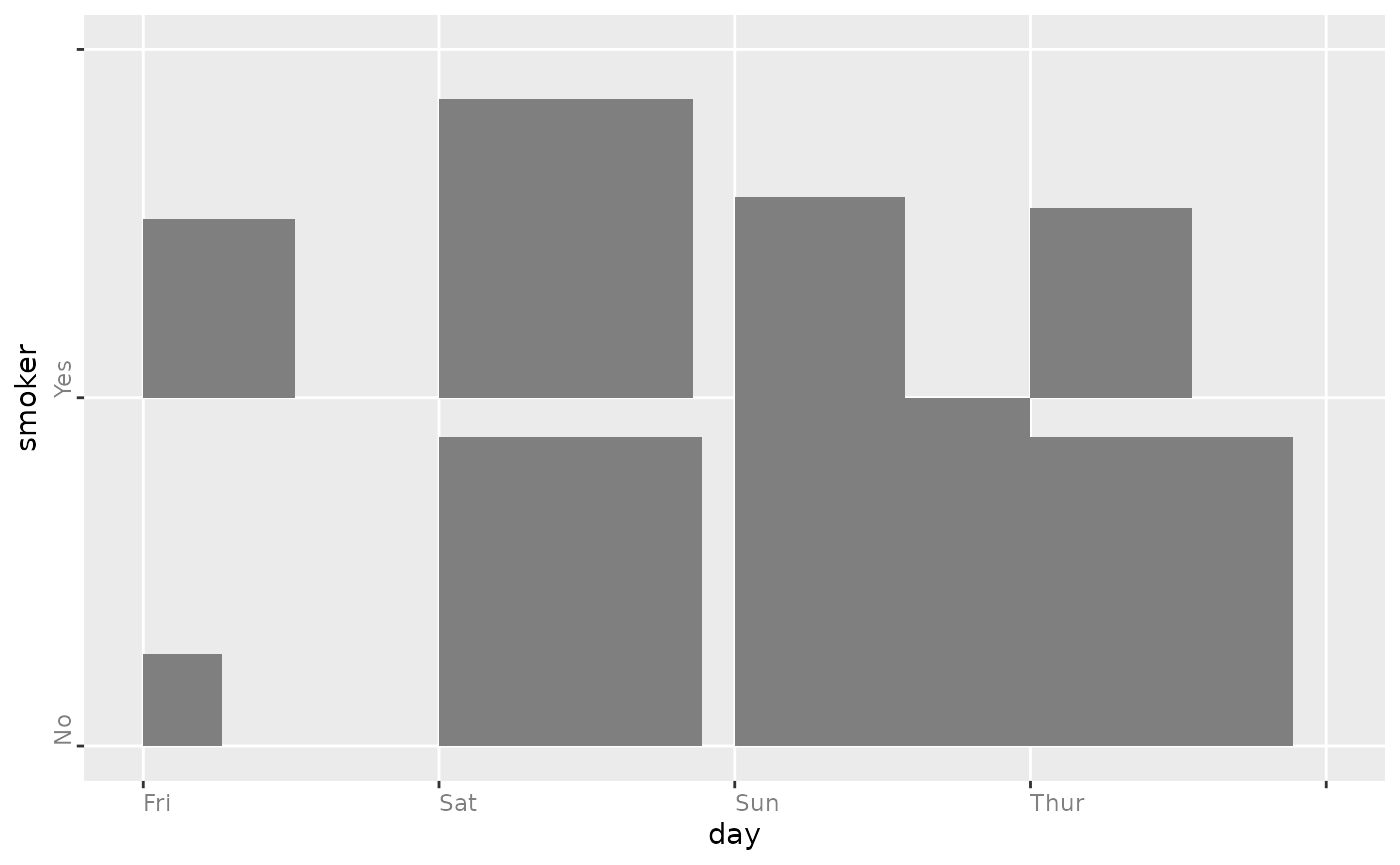
The same mosaic plot of smoker versus day; colouring by time is ignored.

ggally_rowbar()

ggally_rowbar(tips, aes(x = day, y = smoker))
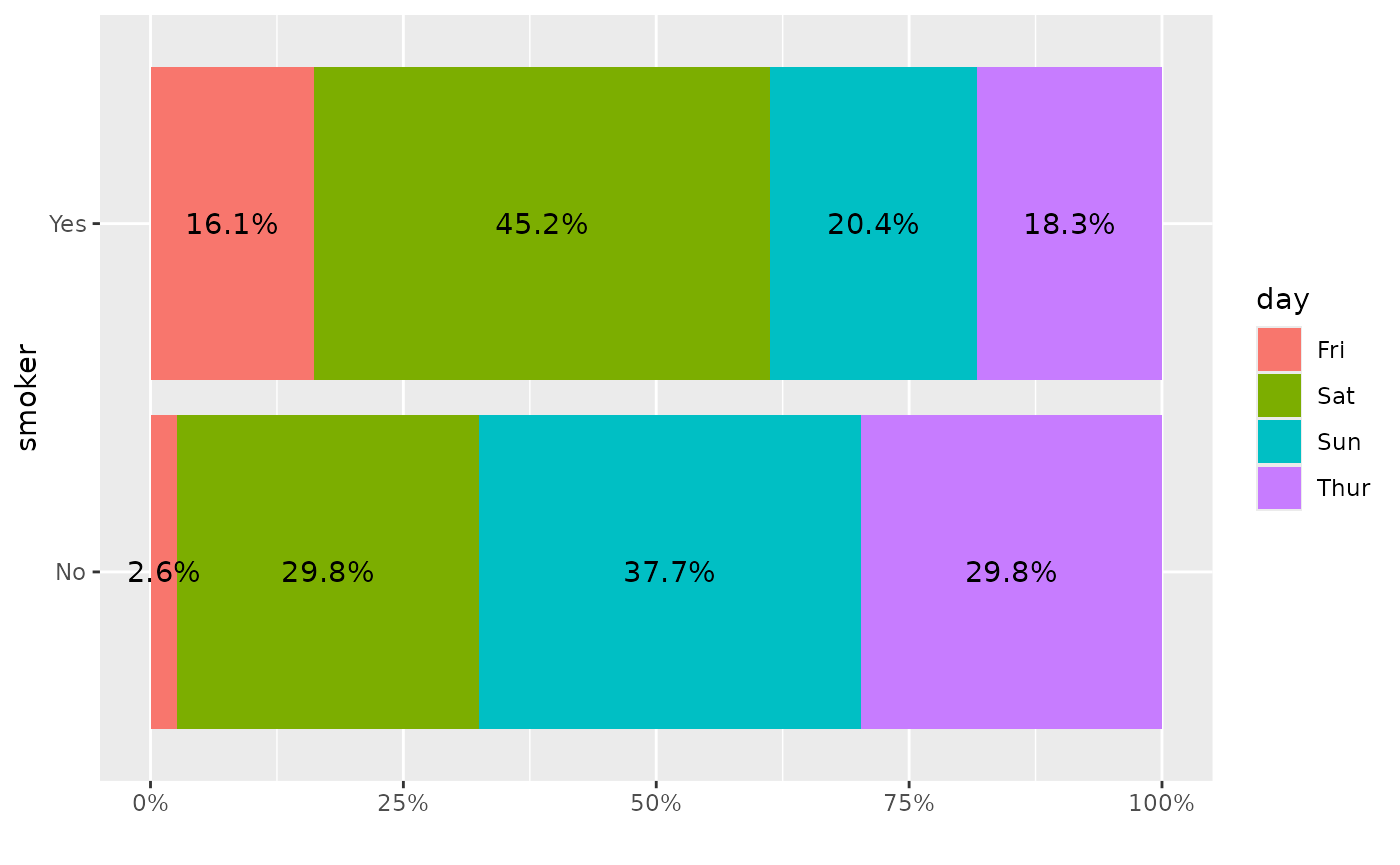
Stacked horizontal bar chart of the percentage of each day within each smoker group, with percent labels. Saturday is the largest share among smokers (45 percent); Sunday is the largest among non-smokers.

Note: the colour aesthetic is not taken into account.

ggally_table()

ggally_table(tips, aes(x = day, y = smoker))
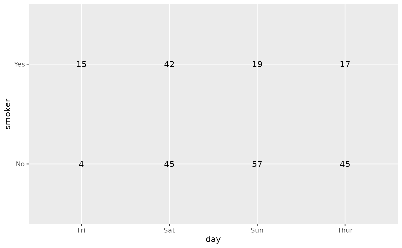
Table of counts of smoker versus day, shown as numbers at each day and smoker position.

ggally_table(tips, aes(x = day, y = smoker, colour = time))
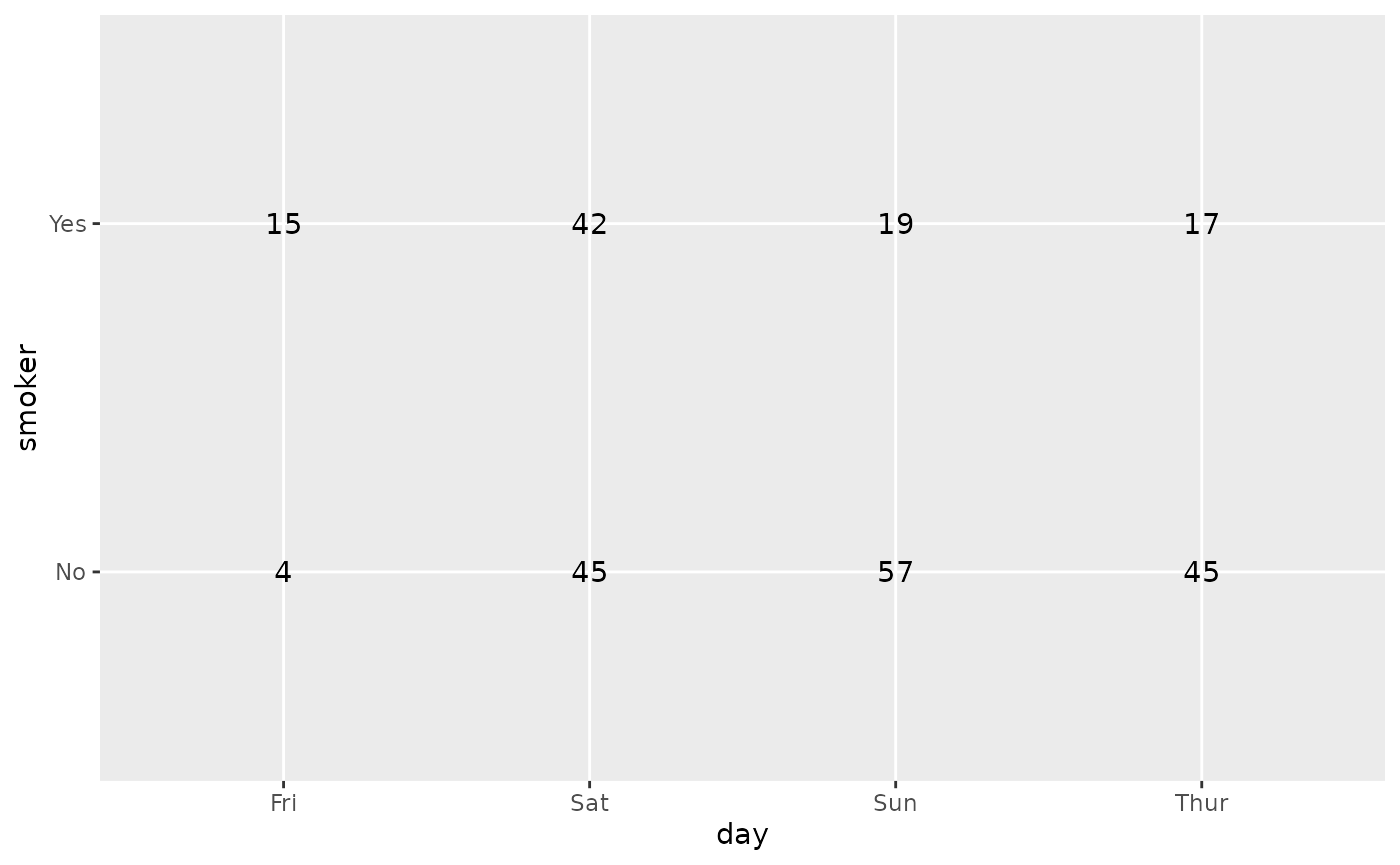
The same table of counts of smoker versus day; colouring by time is ignored.

ggally_table(tips, aes(x = day, y = smoker, colour = smoker))
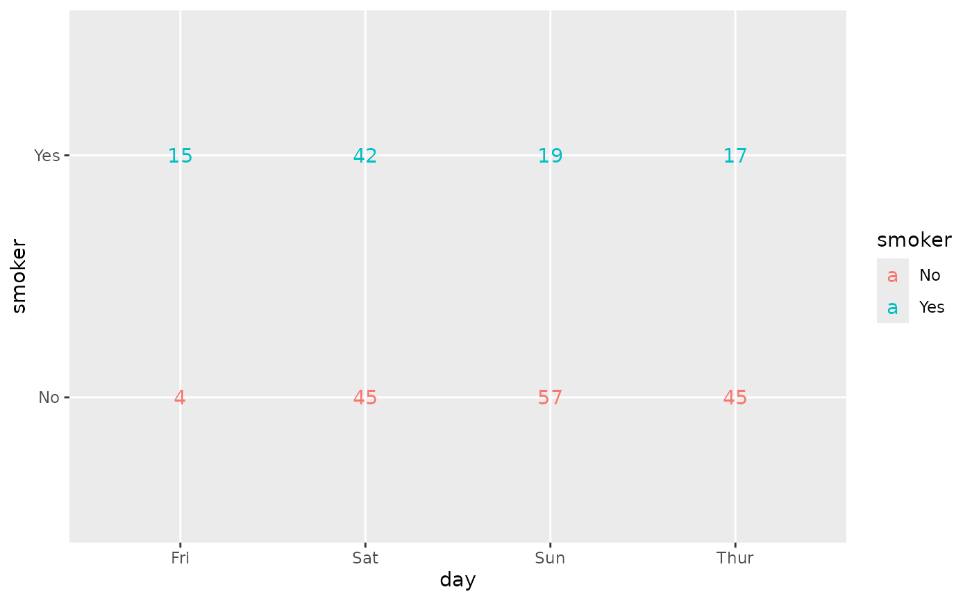
Table of counts of smoker versus day, with numbers coloured by smoker.

Note: colour aesthetic is taken into account only if it corresponds to x or to y.

ggally_trends(tips, aes(x = day, y = smoker))
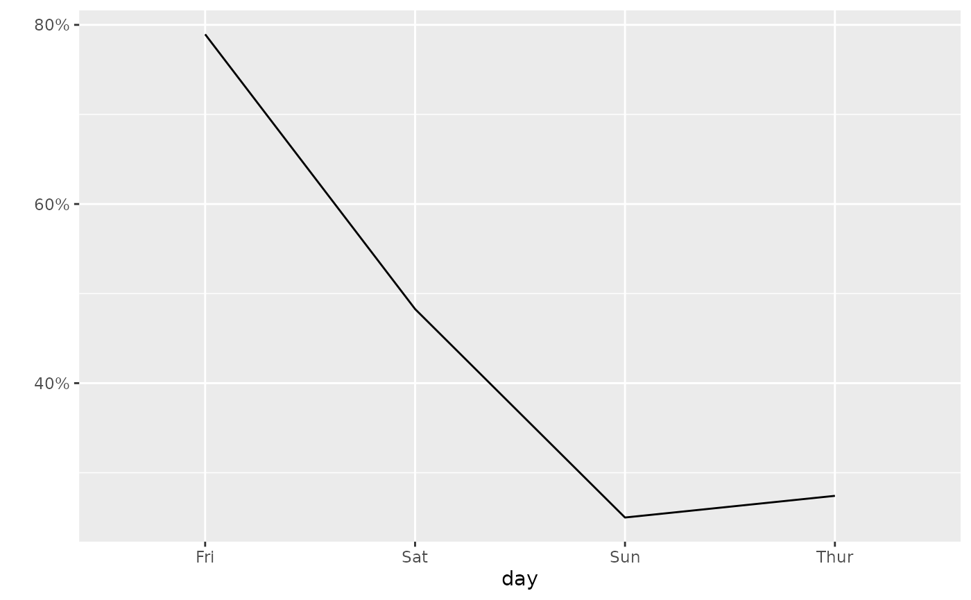
Line chart of the share of smokers by day. It drops from about 79 percent on Friday to about 25 percent on Sunday.

ggally_trends(tips, aes(x = day, y = smoker, colour = time))
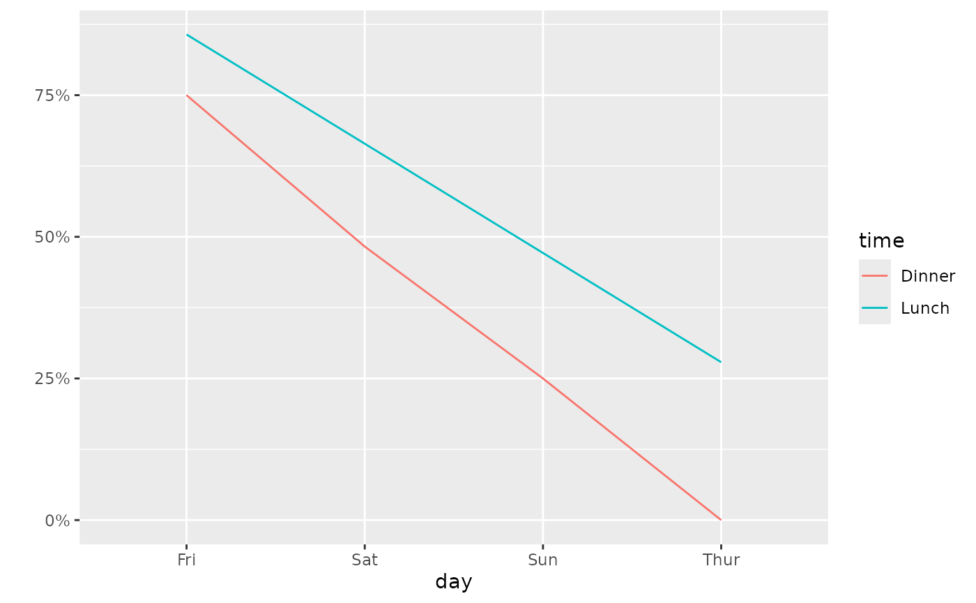
Line chart of the share of smokers by day, with one line per time (dinner or lunch). Both lines fall from Friday to Thursday.

with 1x continuous and 1x discrete variables

ggally_autopoint()

ggally_autopoint(tips, aes(x = total_bill, y = day))
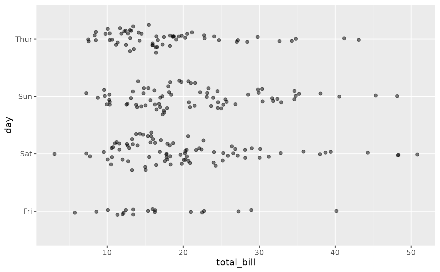
Jittered point plot of day versus total bill. Each day spreads from about 5 to 50 dollars, with most bills between 10 and 25.

ggally_autopoint(tips, aes(x = total_bill, y = day, colour = time))
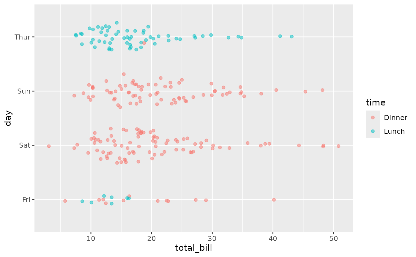
Jittered point plot of day versus total bill, coloured by time. Thursday is almost all lunch and the weekend is all dinner.

ggally_box() & ggally_box_no_facet()

ggally_box(tips, aes(x = total_bill, y = day))
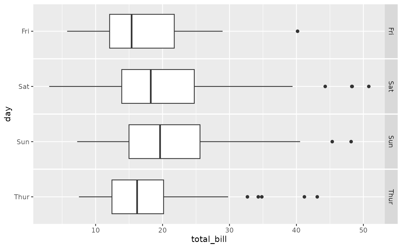
Horizontal boxplots of total bill, one facet per day. Sunday has the highest median bill and Friday the lowest.

ggally_box(tips, aes(x = total_bill, y = day, colour = time))
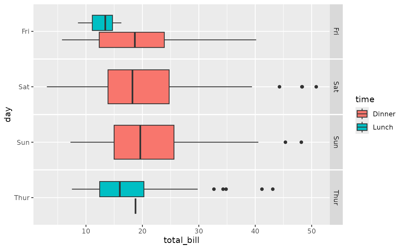
Horizontal boxplots of total bill, one facet per day, split and filled by time. Lunch bills are lower than dinner bills.

ggally_box_no_facet(tips, aes(x = total_bill, y = day))
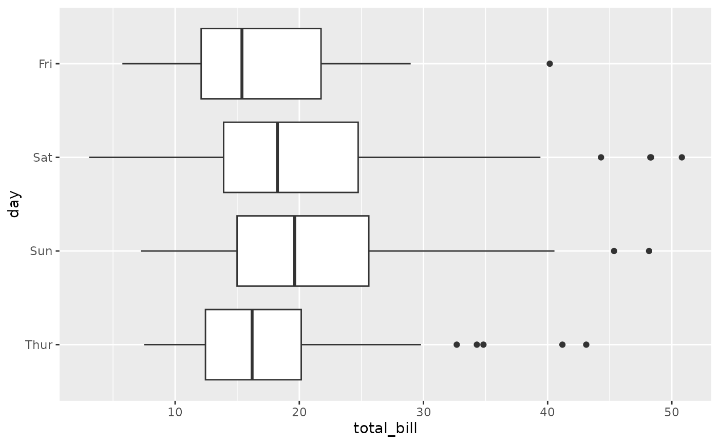
Horizontal boxplots of total bill for each day on one shared panel. Sunday has the highest median bill.

ggally_box_no_facet(tips, aes(x = total_bill, y = day, colour = time))
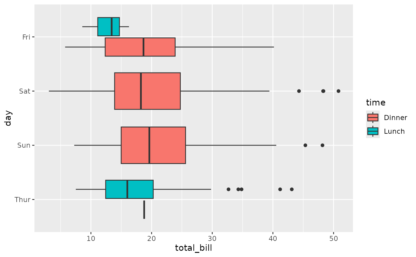
Horizontal boxplots of total bill for each day on one shared panel, split and filled by time. Lunch bills are lower than dinner bills.

ggally_denstrip()

ggally_denstrip(tips, aes(x = total_bill, y = day))
#> `stat_bin()` using `bins = 30`. Pick better value `binwidth`.
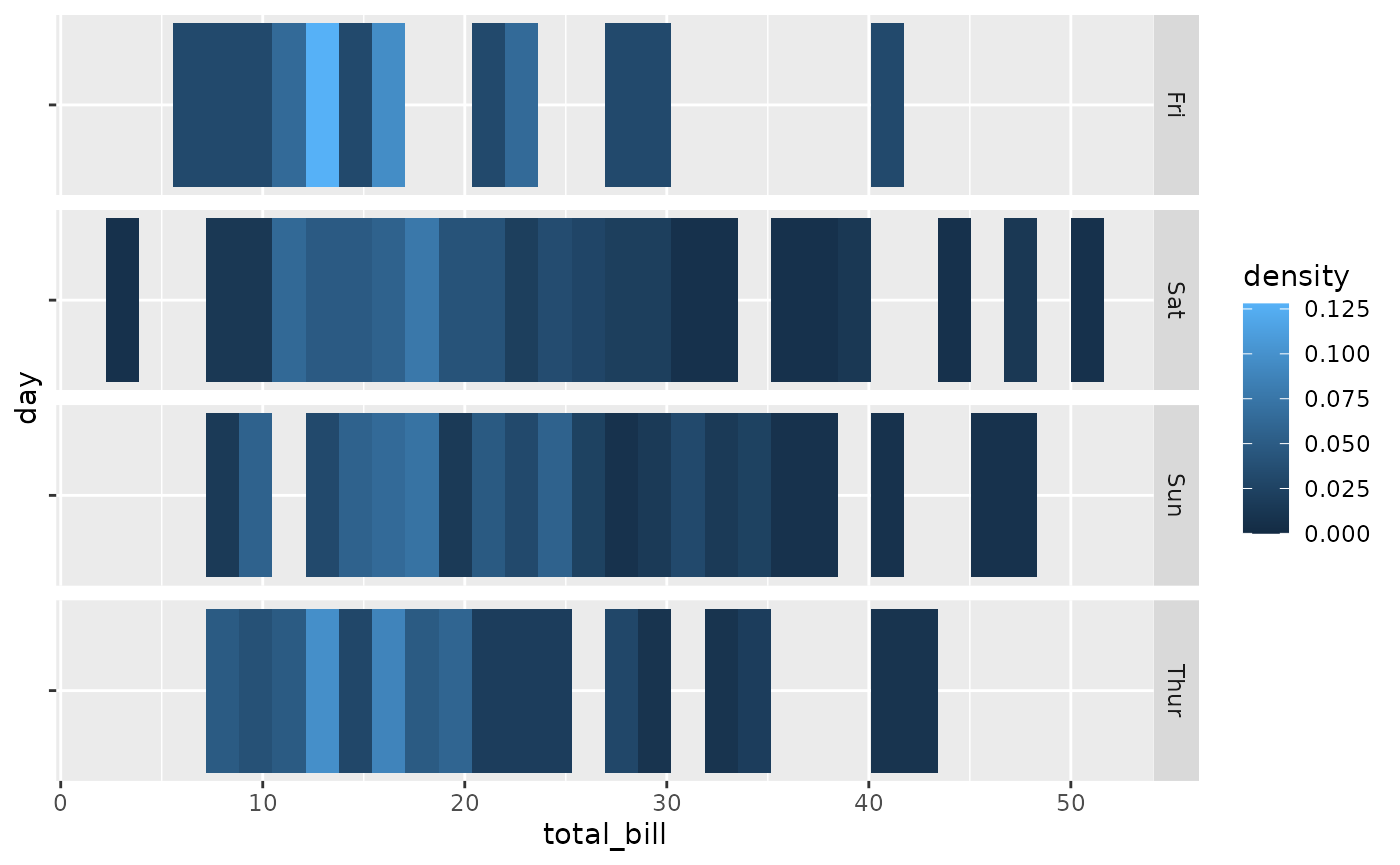
Density strips of total bill, one facet per day, where lighter blue tiles mark denser ranges. Bills cluster between 10 and 25 dollars.

ggally_denstrip(tips, aes(x = total_bill, y = day, colour = time))
#> `stat_bin()` using `bins = 30`. Pick better value `binwidth`.
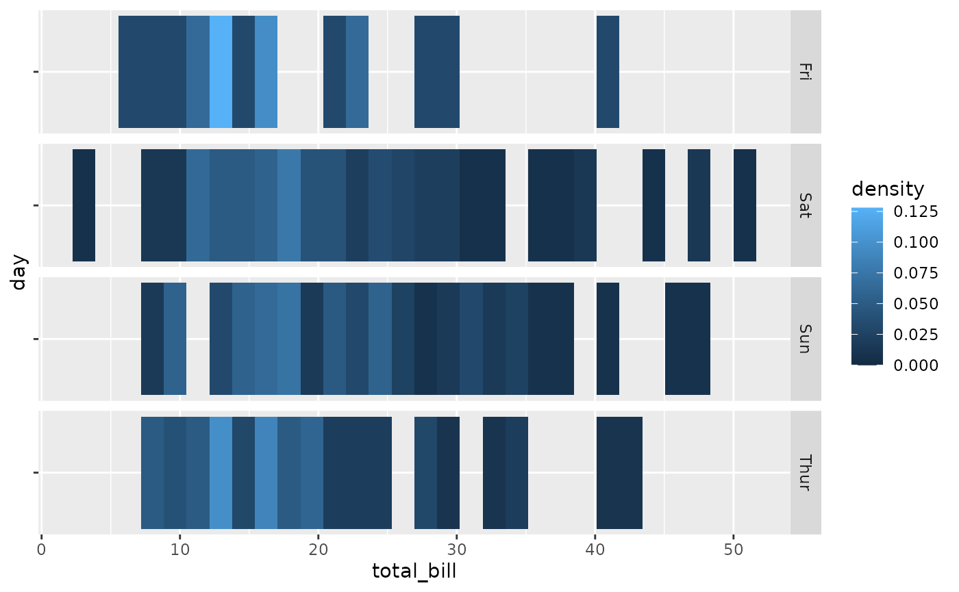
The same density strips of total bill by day; colouring by time is ignored.

ggally_dot() & ggally_dot_no_facet()

ggally_dot(tips, aes(x = total_bill, y = day))
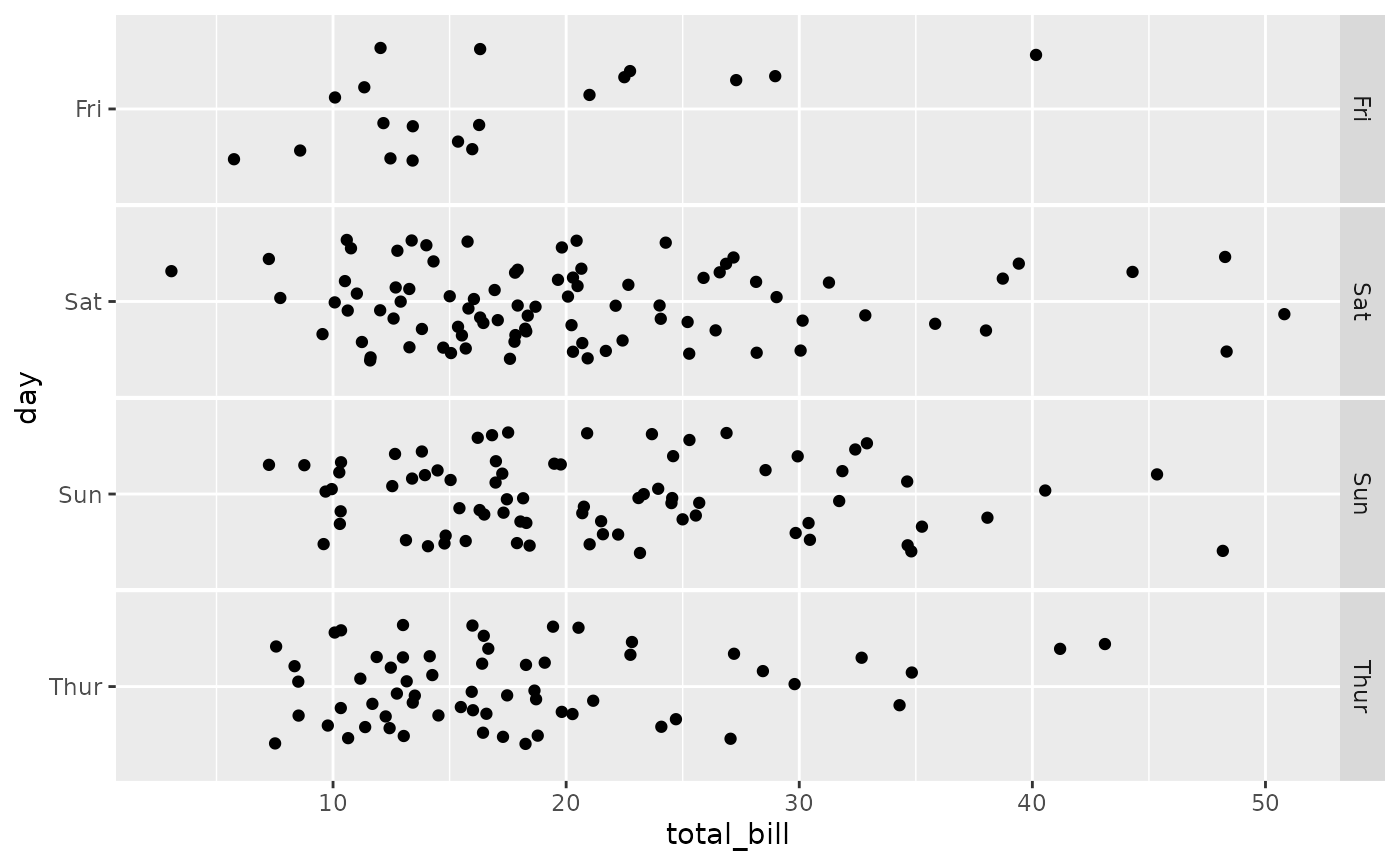
Jittered dot plot of total bill, one facet per day. Bills cluster between 10 and 25 dollars on every day.

ggally_dot(tips, aes(x = total_bill, y = day, colour = time))
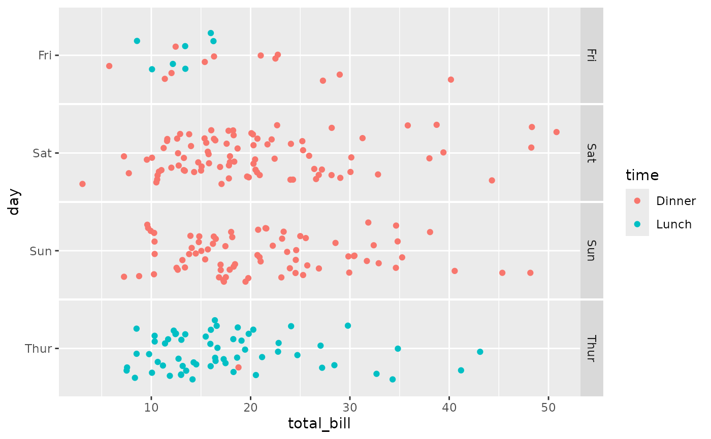
Jittered dot plot of total bill, one facet per day, coloured by time. Thursday is almost all lunch and the weekend is all dinner.

ggally_dot_no_facet(tips, aes(x = total_bill, y = day))
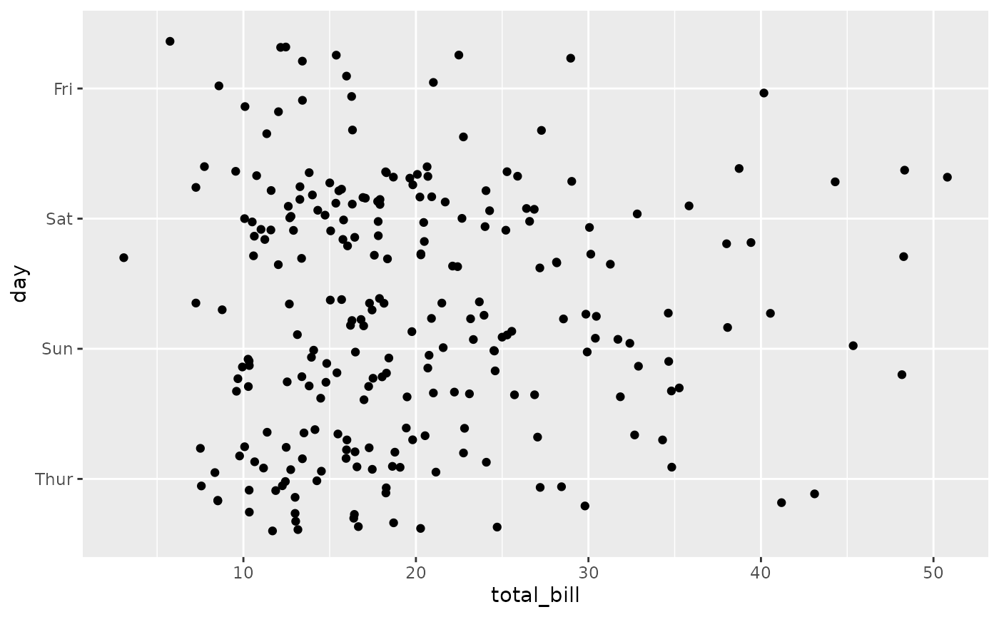
Jittered dot plot of day versus total bill on one shared panel. Bills cluster between 10 and 25 dollars on every day.

ggally_dot_no_facet(tips, aes(x = total_bill, y = day, colour = time))
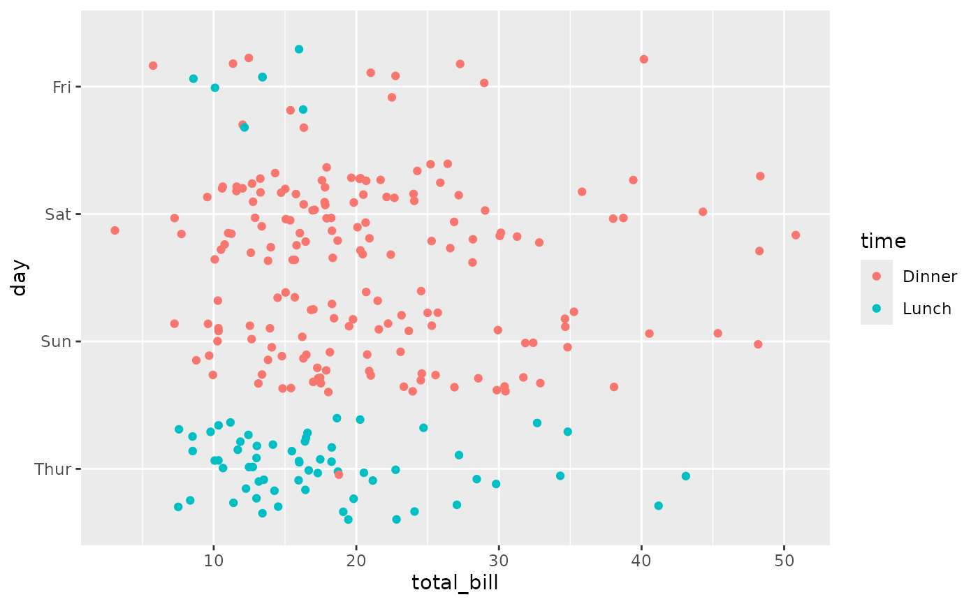
Jittered dot plot of day versus total bill on one shared panel, coloured by time.

ggally_facetdensitystrip()

ggally_facetdensitystrip(tips, aes(x = total_bill, y = day))
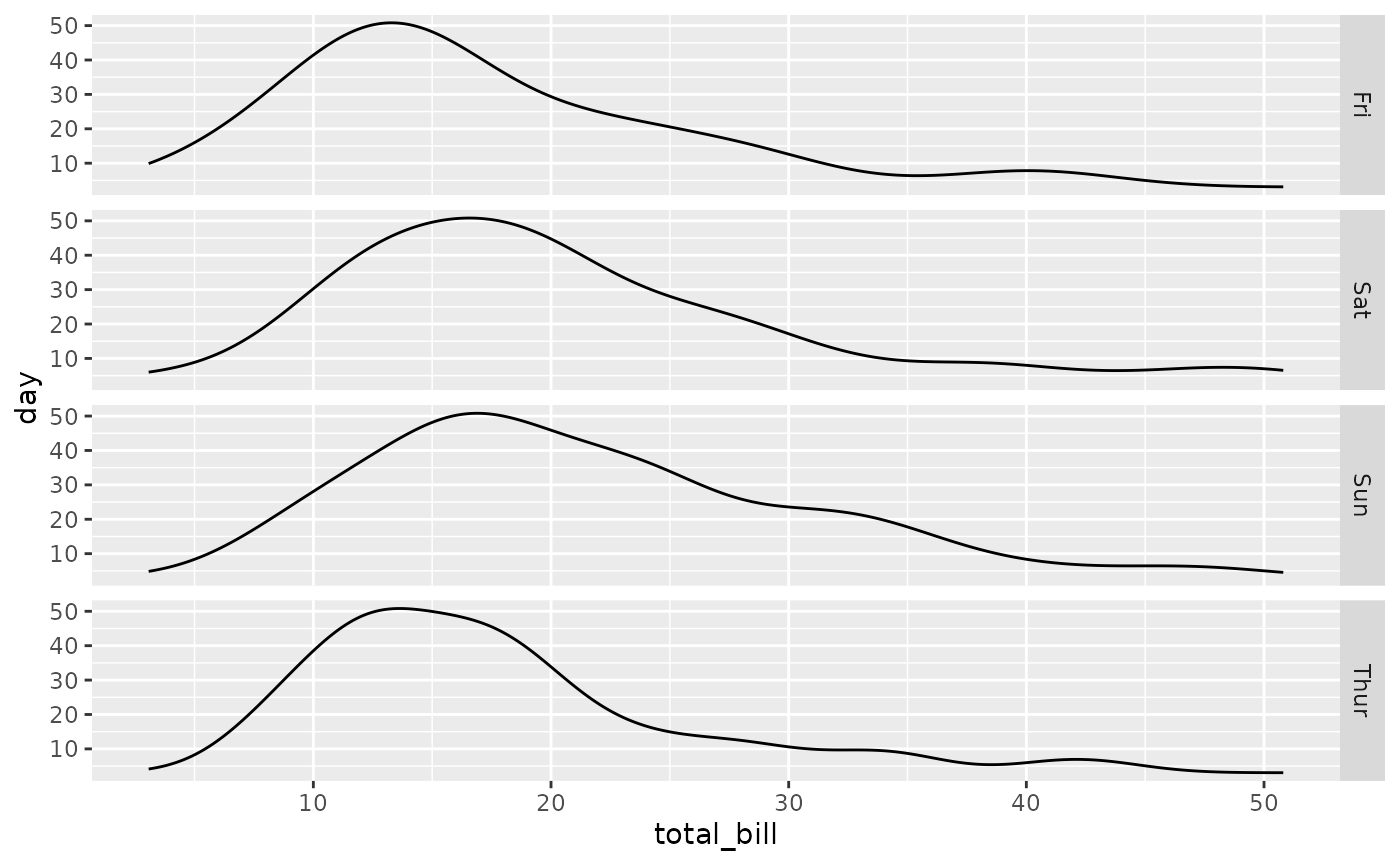
Density curves of total bill, one facet per day. Each curve peaks around 13 to 18 dollars with a long right tail.

ggally_facetdensitystrip(tips, aes(x = total_bill, y = day, colour = time))
#> Warning: Groups with fewer than two data points have been dropped.
#> Warning: Removed 1 row containing missing values or values outside the scale range
#> (`geom_line()`).
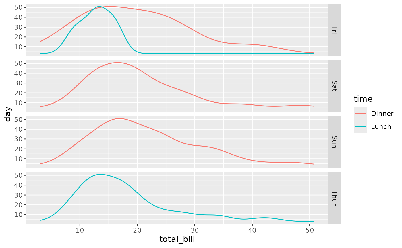
Density curves of total bill, one facet per day, with one curve per time. Friday lunch bills are tightly grouped around 13 dollars.

ggally_facethist()

ggally_facethist(tips, aes(x = total_bill, y = day))
#> `stat_bin()` using `bins = 30`. Pick better value `binwidth`.
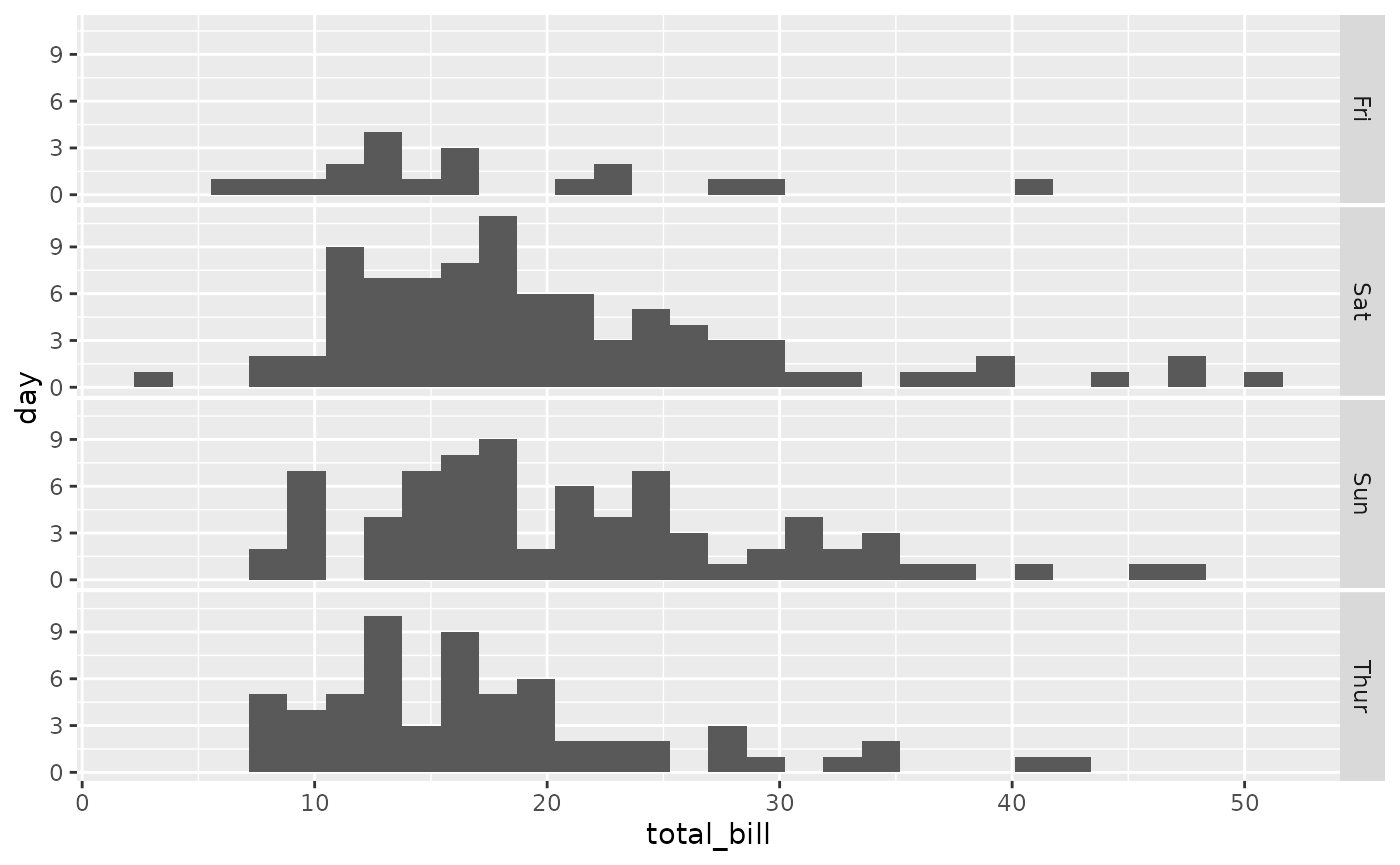
Histograms of total bill, one facet per day. Saturday and Sunday have the most bills, Friday the fewest.

ggally_facethist(tips, aes(x = total_bill, y = day, colour = time))
#> `stat_bin()` using `bins = 30`. Pick better value `binwidth`.
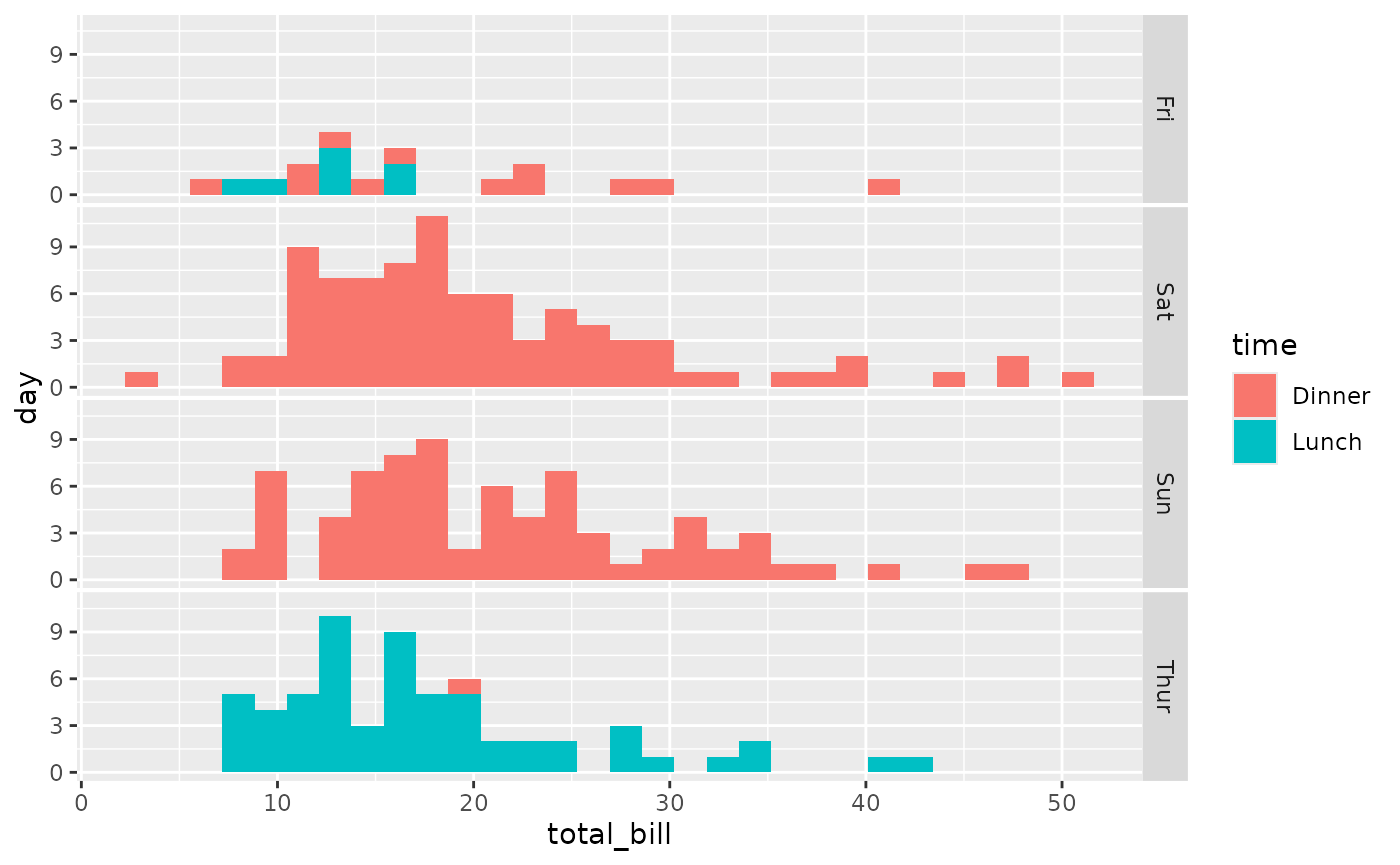
Histograms of total bill, one facet per day, with bars stacked by time. Thursday is almost all lunch and the weekend is all dinner.

ggally_summarise_by()

ggally_summarise_by(tips, aes(x = total_bill, y = day))
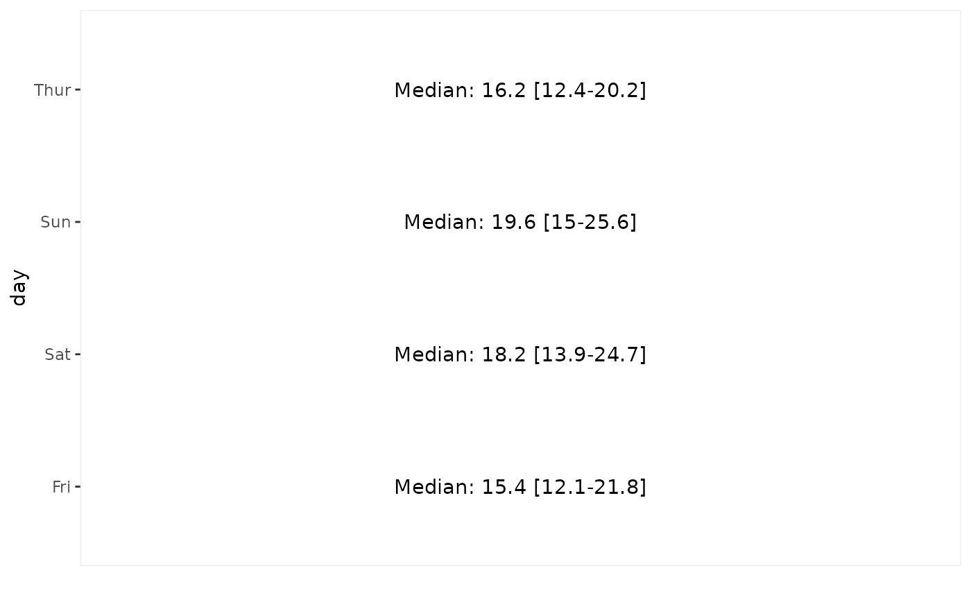
Text panel listing the median total bill and interquartile range for each day. Sunday has the highest median (19.6) and Friday the lowest (15.4).

ggally_summarise_by(tips, aes(x = total_bill, y = day, colour = day))
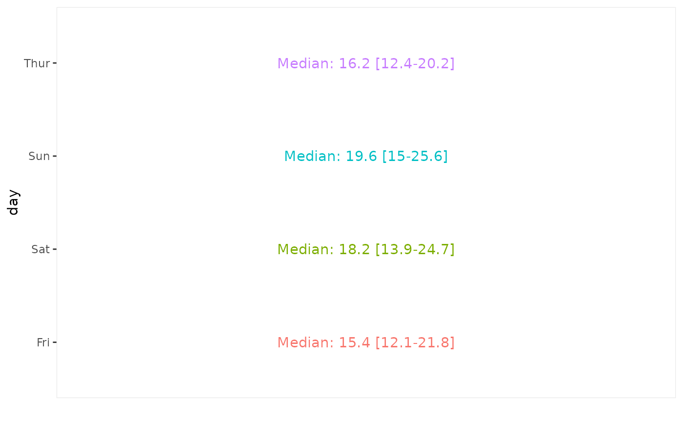
The same median and interquartile range text for each day, with each day's text in its own colour.

Note: colour aesthetic is kept only if corresponding to the discrete axis.

ggally_trends(tips, aes(y = total_bill, x = day))
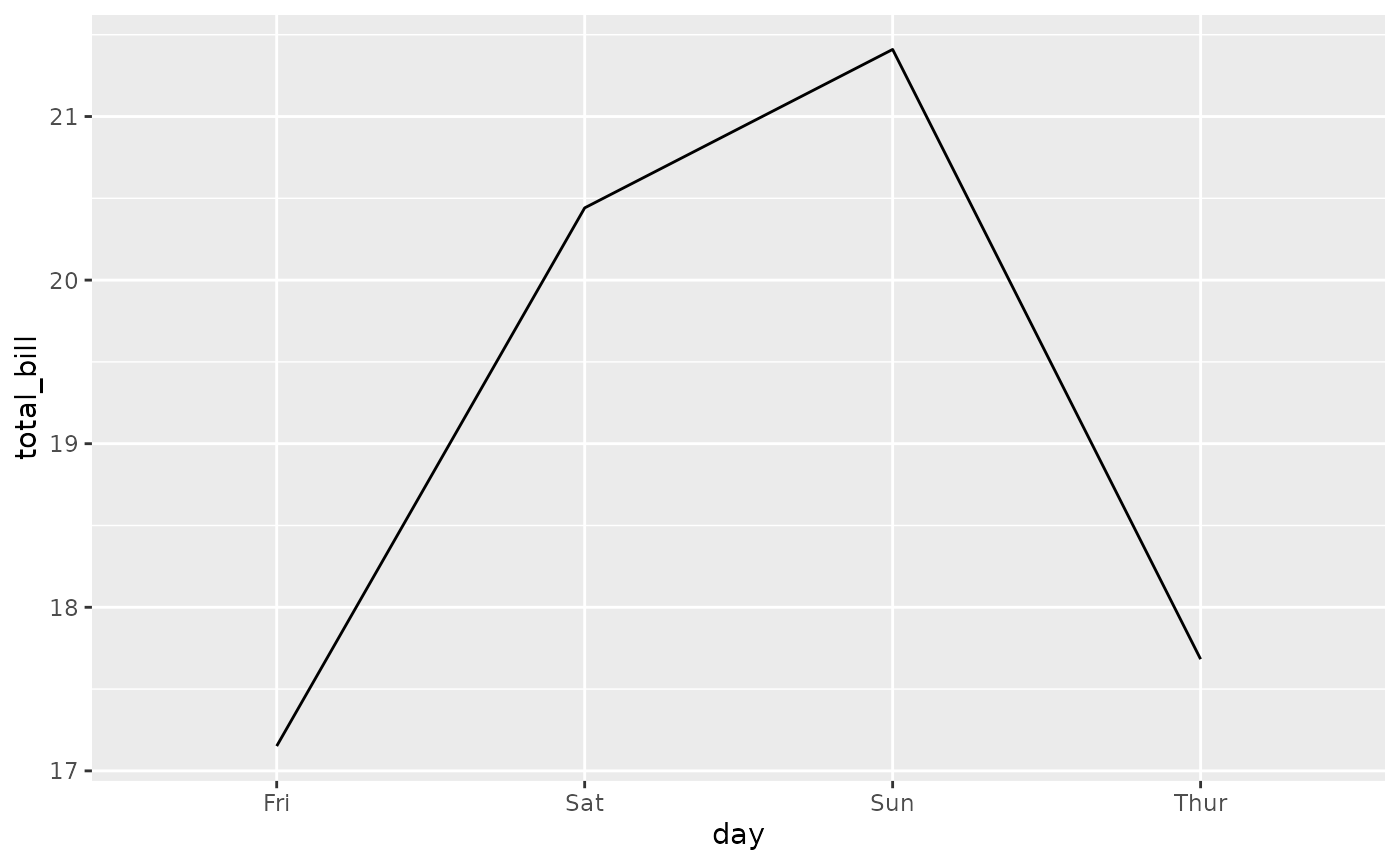
Line chart of mean total bill by day. It rises from about 17 dollars on Friday to about 21 on Sunday, then drops on Thursday.

ggally_trends(tips, aes(y = total_bill, x = day, colour = time))
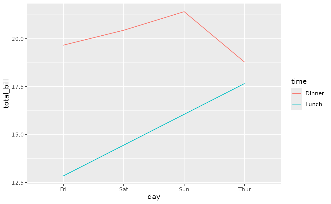
Line chart of mean total bill by day, with one line per time. Dinner bills are higher than lunch bills on every day.

Diagonal plots

with 1x continuous variable

ggally_autopointDiag()

ggally_autopointDiag(tips, aes(x = total_bill))
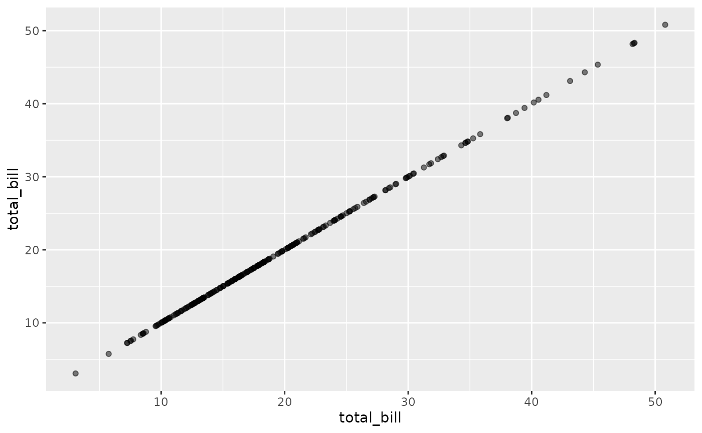
Points of total bill plotted against itself, forming a straight diagonal line.

ggally_autopointDiag(tips, aes(x = total_bill, colour = time))
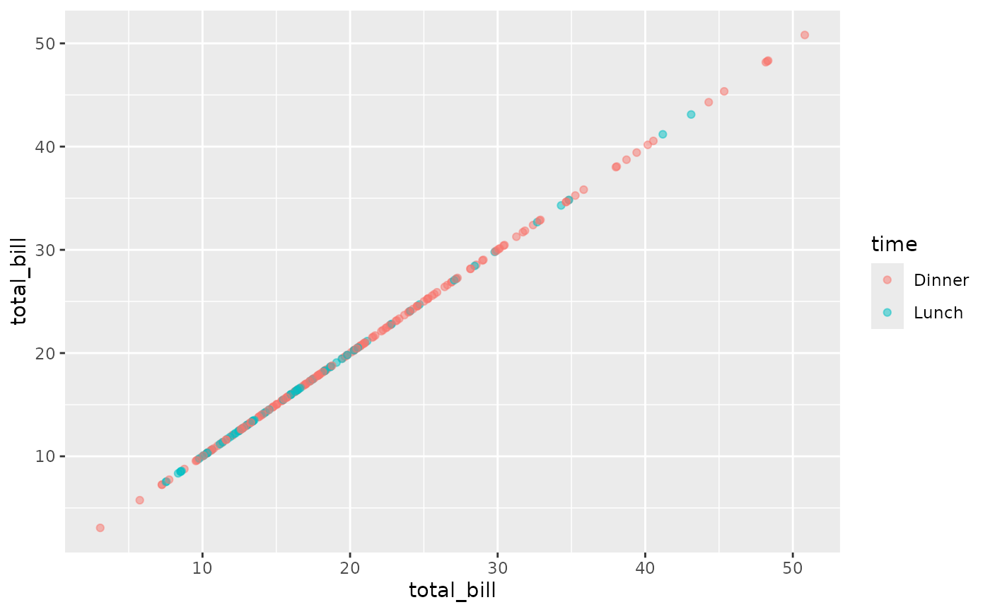
Points of total bill plotted against itself, forming a straight diagonal line, coloured by time.

ggally_barDiag()

ggally_barDiag(tips, aes(x = total_bill))
#> `stat_bin()` using `bins = 30`. Pick better value `binwidth`.
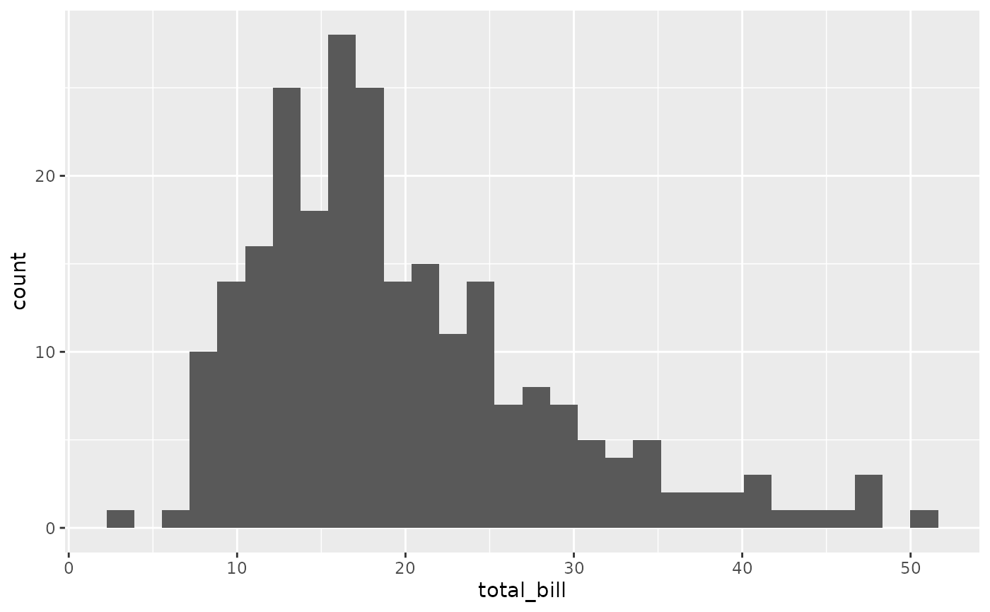
Histogram of total bill. It is right skewed, with most bills between 10 and 25 dollars.

ggally_barDiag(tips, aes(x = total_bill, colour = time))
#> `stat_bin()` using `bins = 30`. Pick better value `binwidth`.
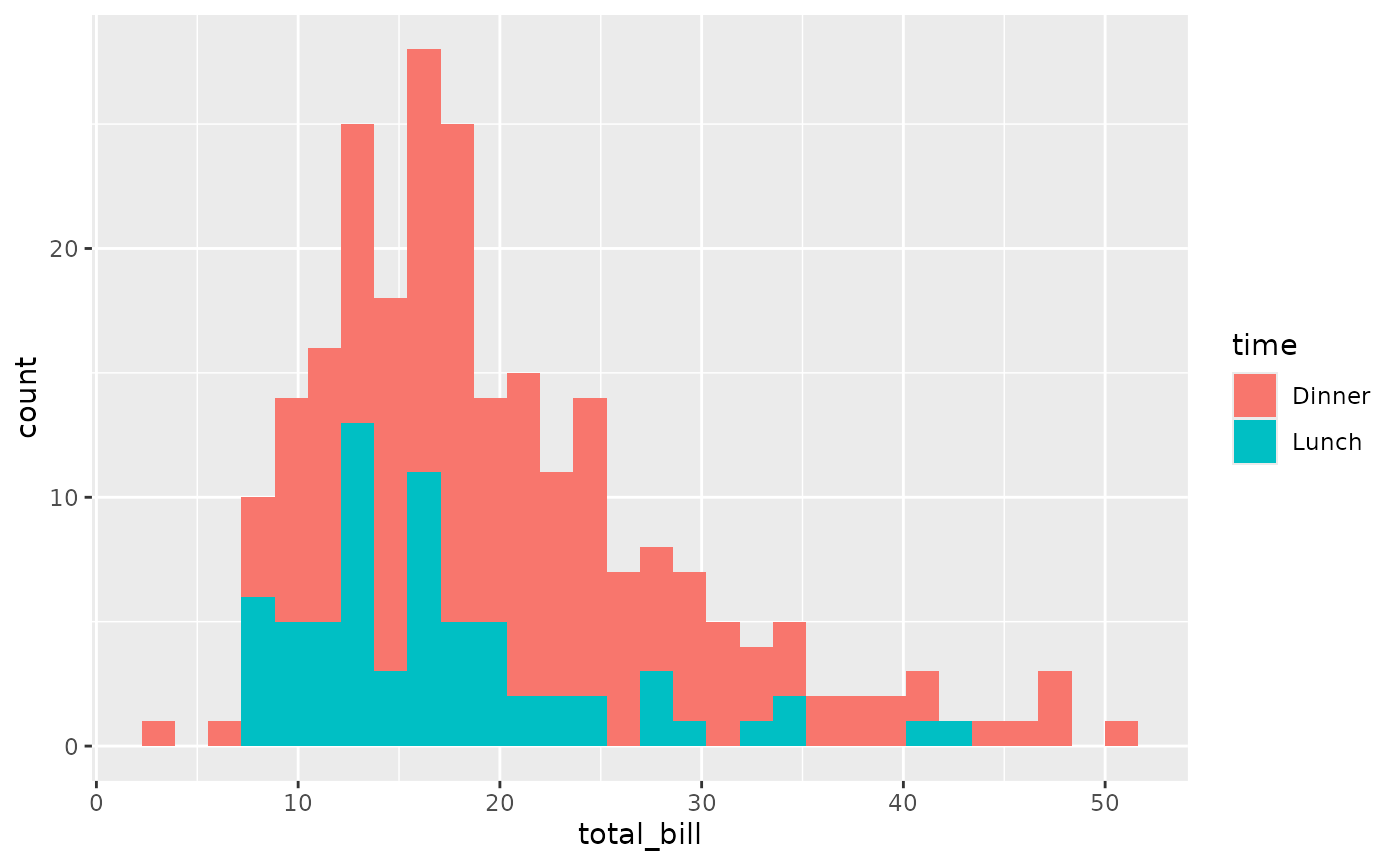
Histogram of total bill with bars stacked by time. Lunch bills sit at the lower end.

ggally_densityDiag()

ggally_densityDiag(tips, aes(x = total_bill))
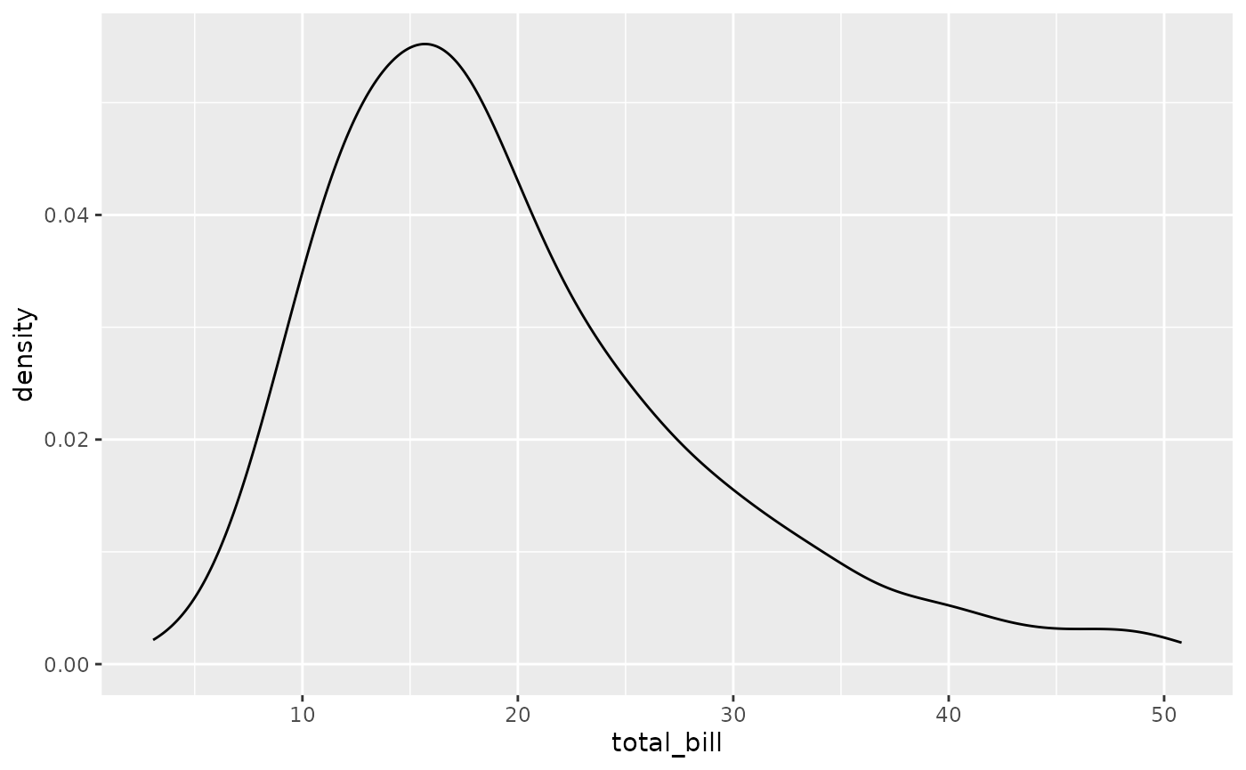
Density curve of total bill. It peaks near 16 dollars and has a long right tail.

ggally_densityDiag(tips, aes(x = total_bill, colour = time))
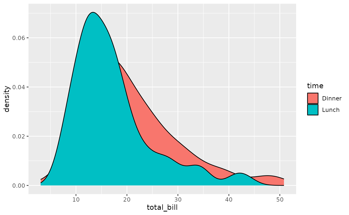
Density curves of total bill filled by time. The lunch curve peaks at a lower bill and is narrower than dinner.

with 1x discrete variable

ggally_autopointDiag()

ggally_autopointDiag(tips, aes(x = day))
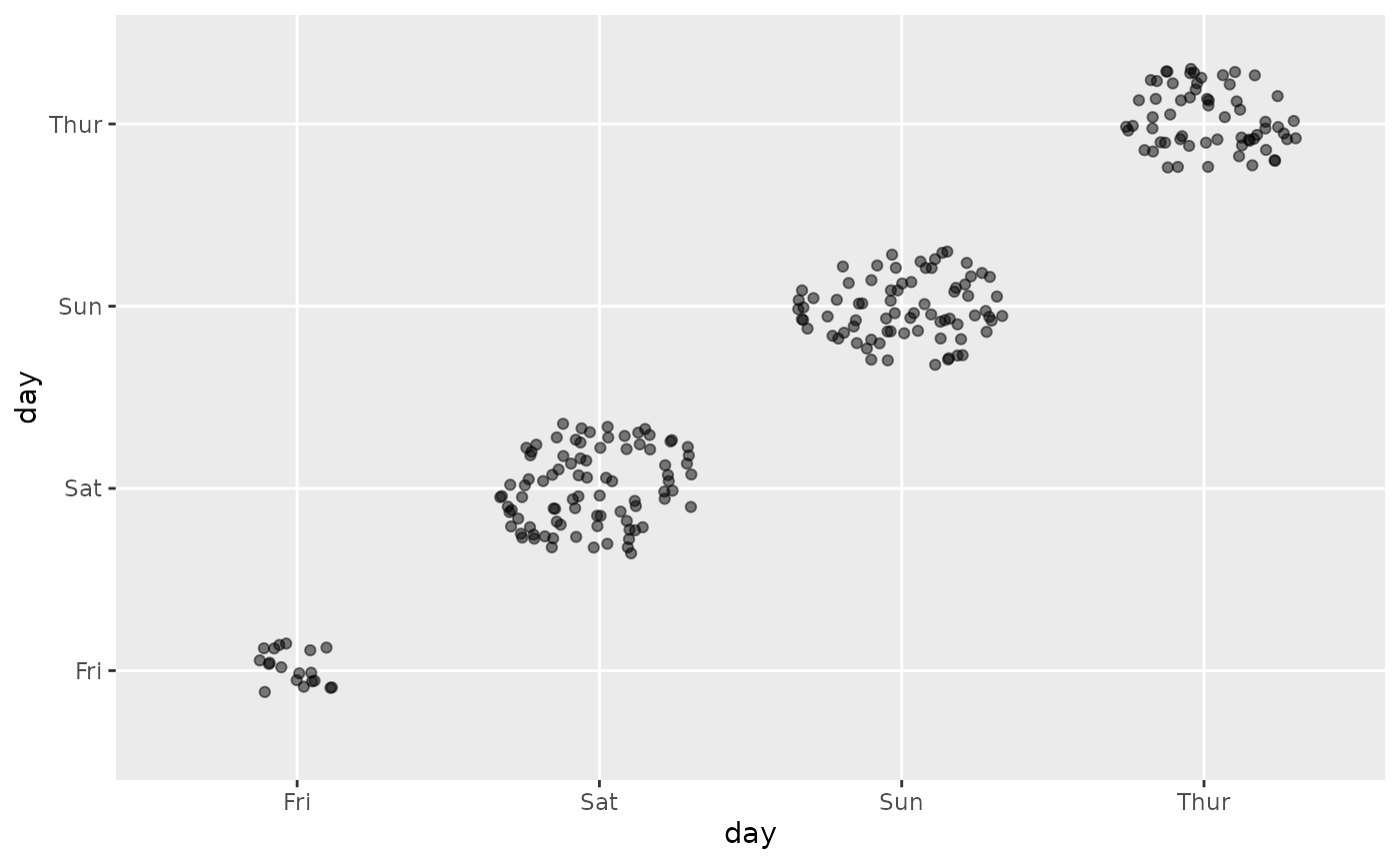
Jittered point clouds of day against itself, placed along the diagonal. Saturday and Sunday have the largest clouds, Friday the smallest.

ggally_autopointDiag(tips, aes(x = day, colour = time))
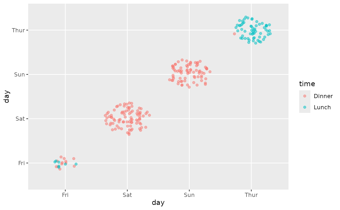
Jittered point clouds of day against itself along the diagonal, coloured by time. Thursday is lunch and the weekend is dinner.

ggally_barDiag()

ggally_barDiag(tips, aes(x = day))
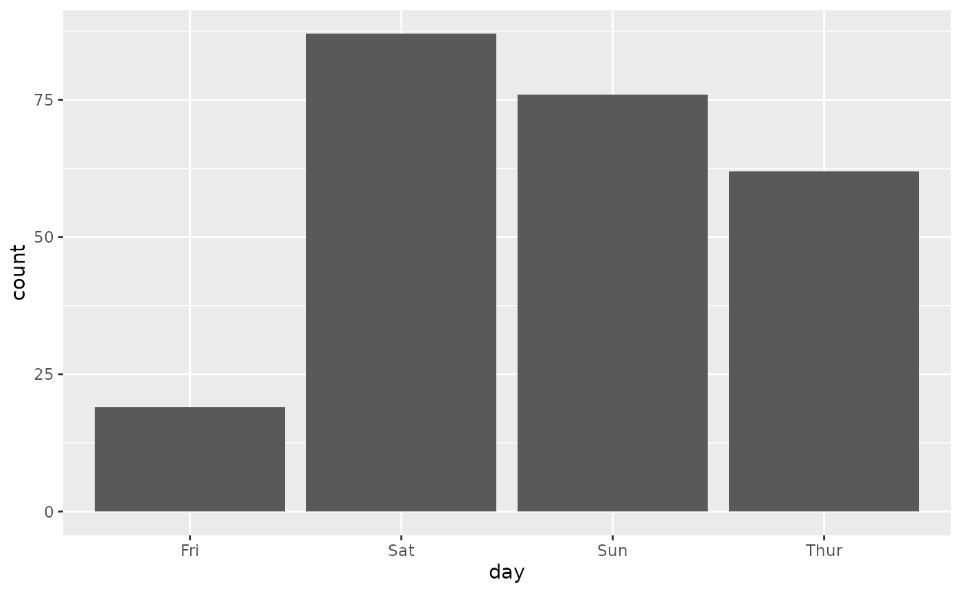
Bar chart of bill counts by day. Saturday has the most bills and Friday the fewest.

ggally_barDiag(tips, aes(x = day, colour = time))
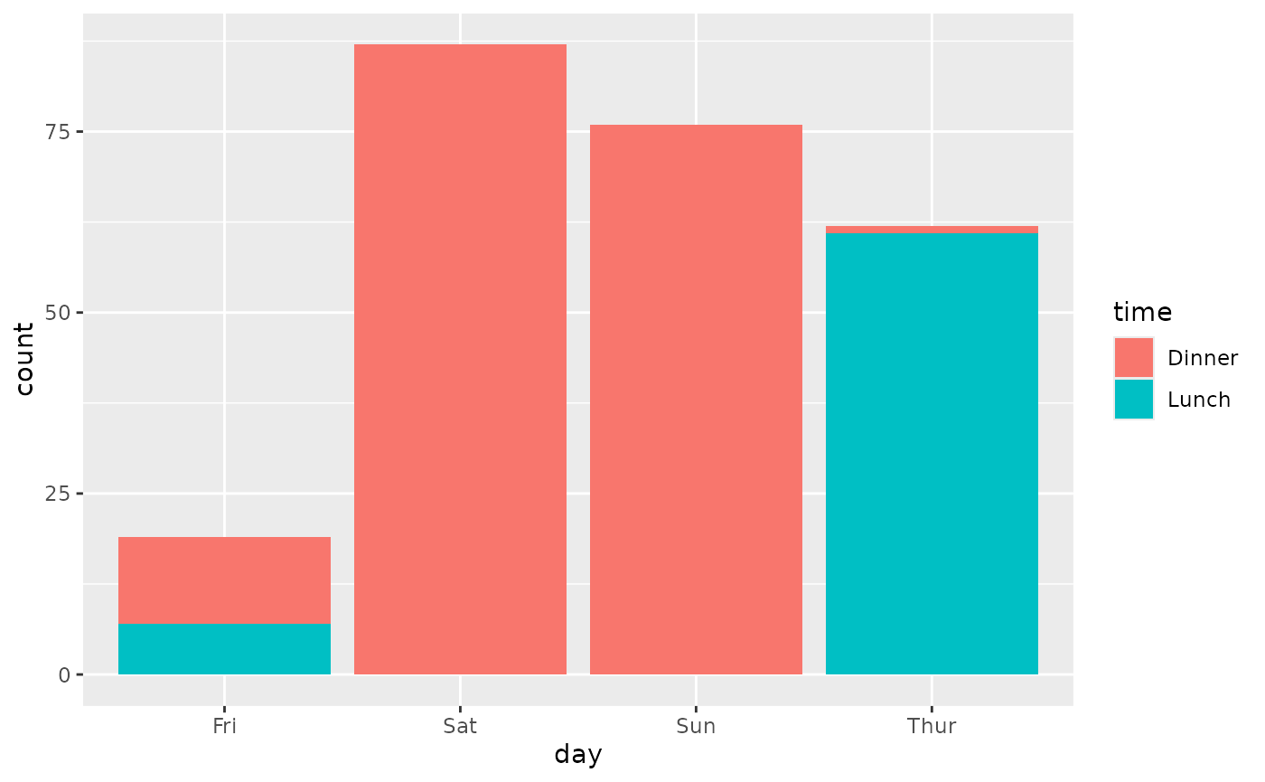
Bar chart of bill counts by day, stacked by time. Thursday is almost all lunch and the weekend is all dinner.

ggally_countDiag()

ggally_countDiag(tips, aes(x = day))
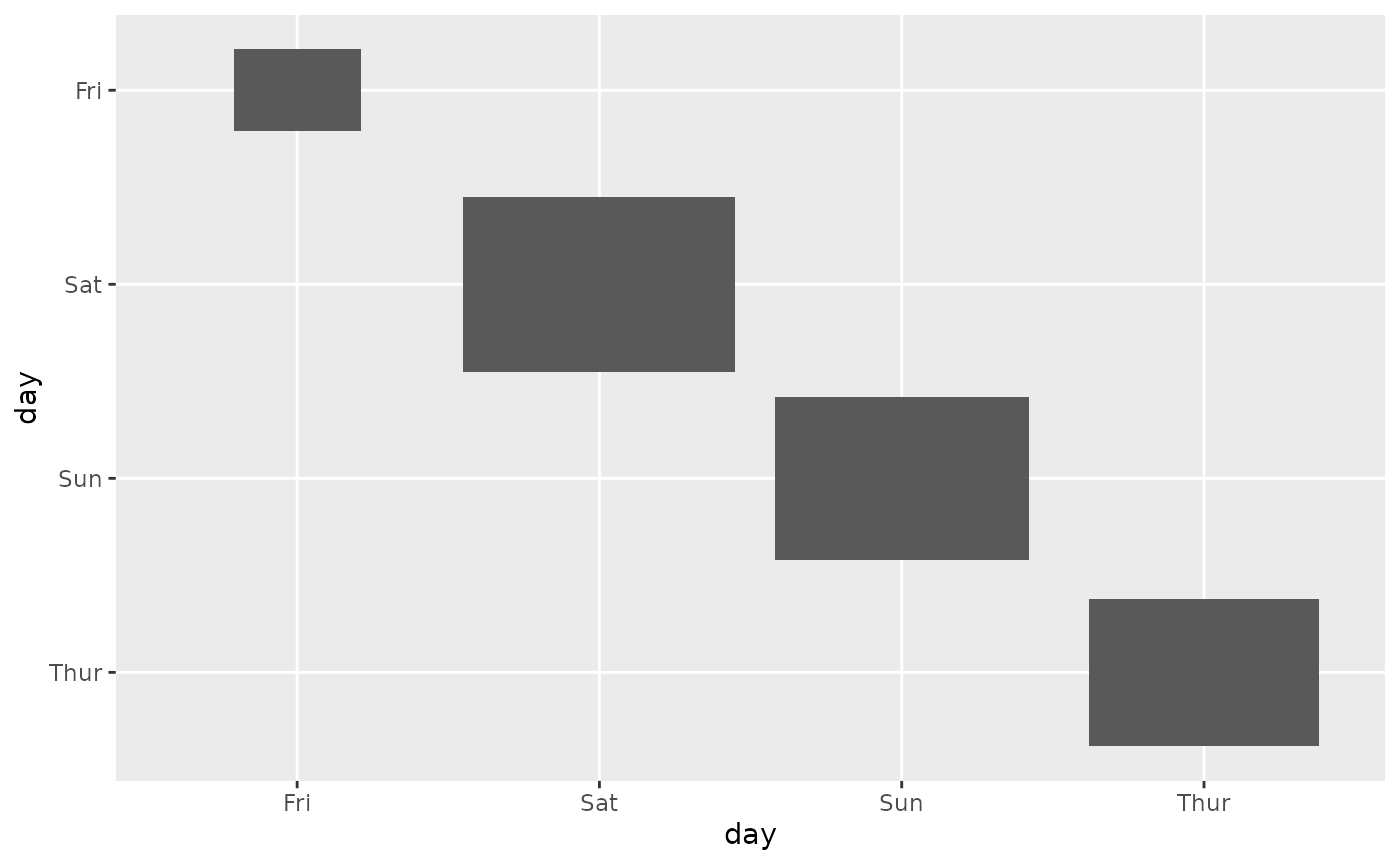
Grey squares of day against itself along the diagonal, sized by count. Saturday is the largest and Friday the smallest.

ggally_countDiag(tips, aes(x = day, colour = time))
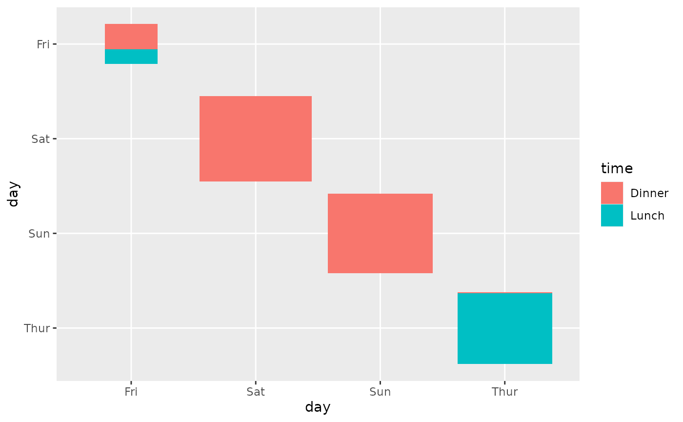
Squares of day against itself along the diagonal, sized by count and filled by time. Thursday is lunch and the weekend is dinner.

ggally_densityDiag()

ggally_densityDiag(tips, aes(x = day))
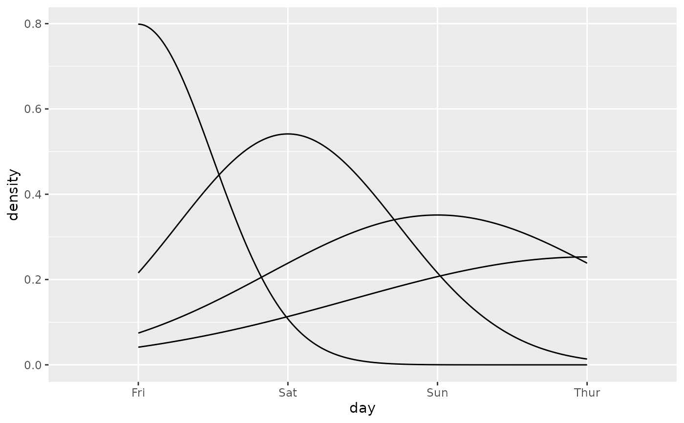
Density curves drawn over the day categories, one curve per day, each peaking at its own day.

ggally_densityDiag(tips, aes(x = day, colour = time))
#> Warning: Groups with fewer than two data points have been dropped.
#> Warning: Removed 1 row containing missing values or values outside the scale range
#> (`geom_density()`).
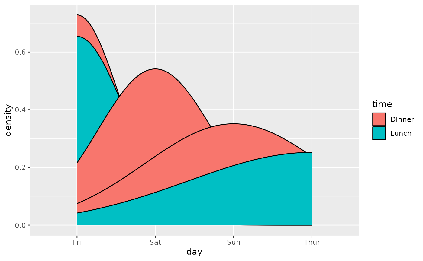
Density curves over the day categories, stacked and filled by time. Lunch dominates Friday and Thursday, dinner dominates Saturday and Sunday.

Additional plots