Skip to contents
library(GGally)
#> Loading required package: ggplot2

GGally::ggbivariate()

The purpose of this function is to easily plot a visualization of the bivariate relation between one outcome and several explanatory variables.

Basic example

Simply indicate the outcome and the explanatory variables. Both could be discrete or continuous.

data(tips)
ggbivariate(tips, outcome = "smoker", explanatory = c("day", "time", "sex", "tip"))
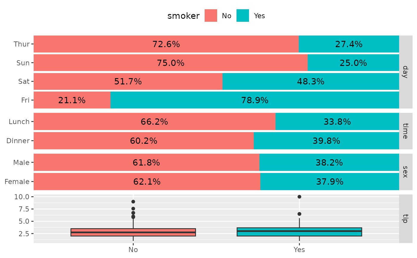
Column of four plots showing smoker status against day, time, sex, and tip. Stacked percentage bars for day, time, and sex show Friday has the highest share of smokers, and a box plot shows tip by smoker status.

ggbivariate(tips, outcome = "total_bill", explanatory = c("day", "time", "sex", "tip"))
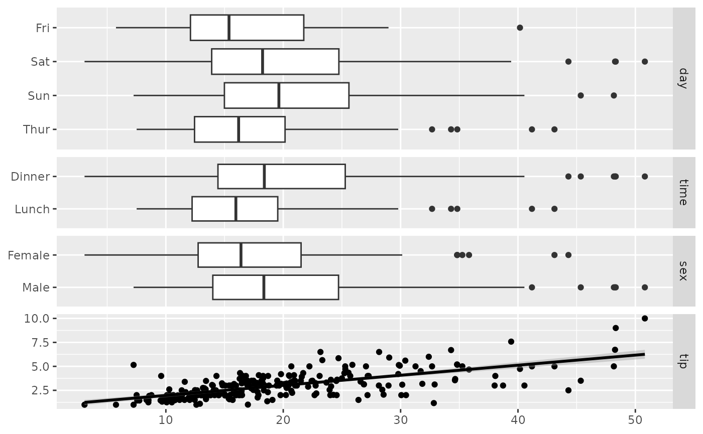
Column of four plots showing total bill against day, time, sex, and tip. Box plots show higher bills on weekends, at dinner, and for men, and a scatterplot shows tip rising with the total bill.

If no explanatory variables are provided, will take all available variables other than the outcome.

ggbivariate(tips, "smoker")
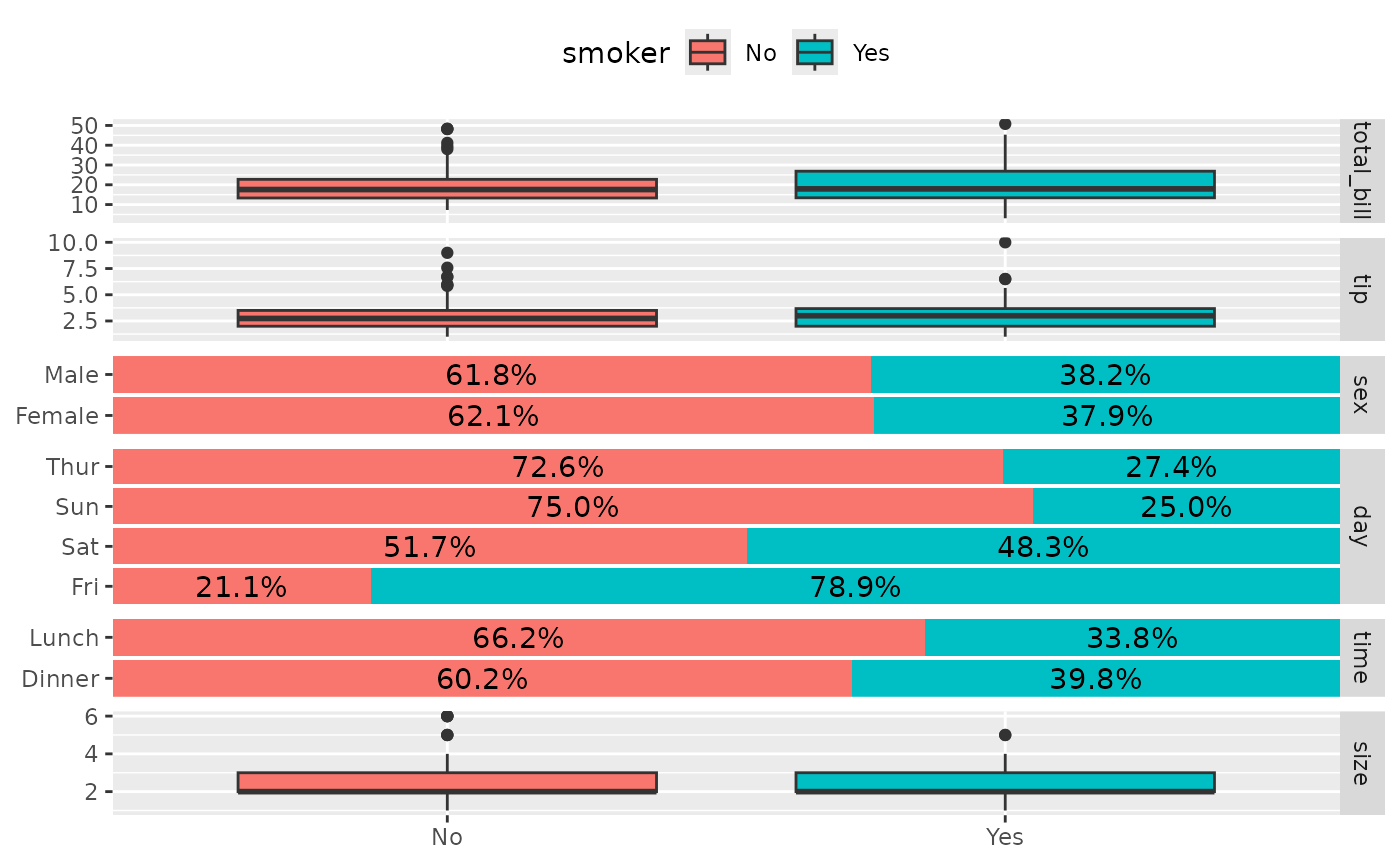
Column of six plots showing smoker status against every other tips variable: total bill, tip, sex, day, time, and size. Discrete variables are stacked percentage bars filled by smoker status and continuous variables are box plots split by smoker status.

Customize plot title and legend title

ggbivariate(
  tips, "smoker", c("day", "time", "sex", "tip"),
  title = "Custom title"
) +
  labs(fill = "Smoker ?")
#> Ignoring unknown labels:
#> • fill : "Smoker ?"
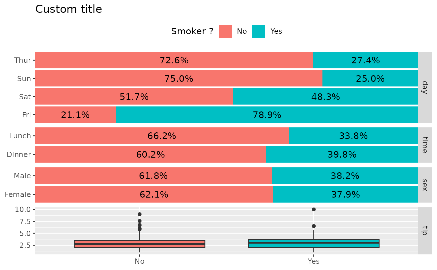
Column of four plots showing smoker status against day, time, sex, and tip, with the title "Custom title" and the legend titled "Smoker ?".

Customize fill colour scale

ggbivariate(tips, "smoker", c("day", "time", "sex", "tip")) +
  scale_fill_brewer(type = "qual")
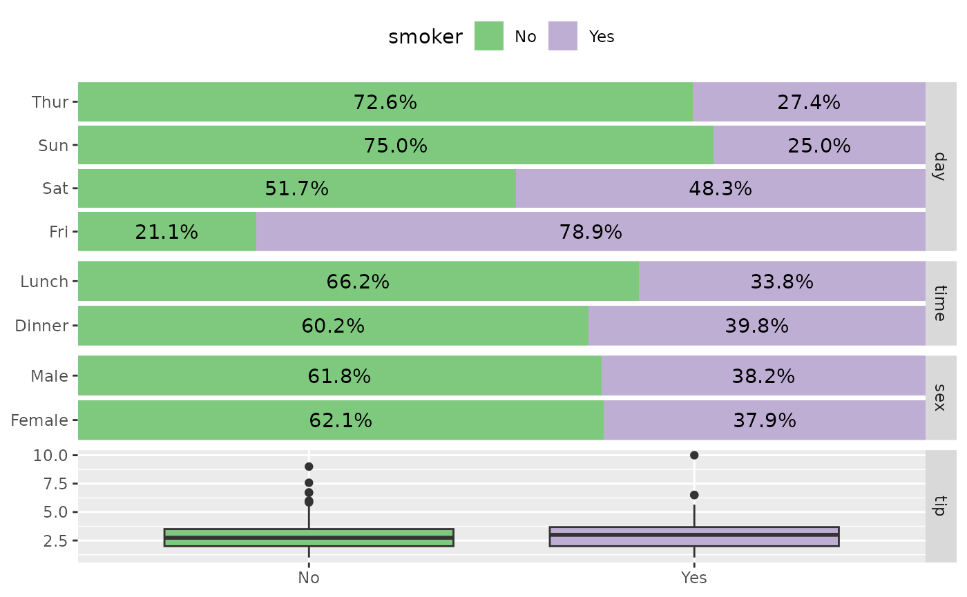
Column of four plots showing smoker status against day, time, sex, and tip, with the stacked percentage bars filled using a qualitative ColorBrewer palette.

Customize labels

ggbivariate(
  tips, "smoker", c("day", "time", "sex", "tip"),
  rowbar_args = list(
    colour = "white",
    size = 4,
    fontface = "bold",
    label_format = scales::label_percent(accurary = 1)
  )
)
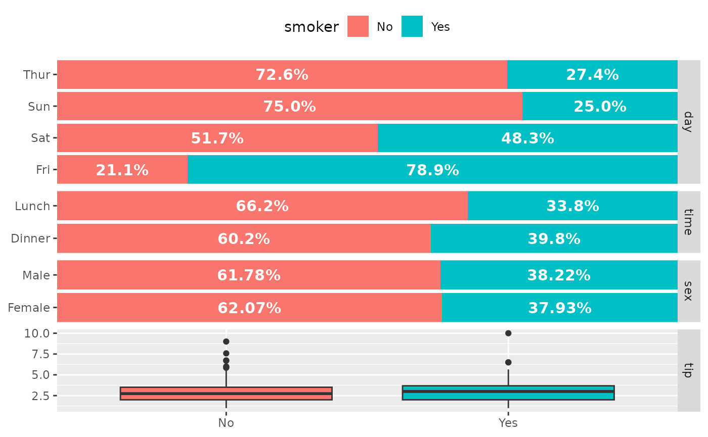
Column of four plots showing smoker status against day, time, sex, and tip, with the percentage labels on the stacked bars drawn in larger bold white text.

Choose the sub-plot from which to get the legend

ggbivariate(tips, "smoker")
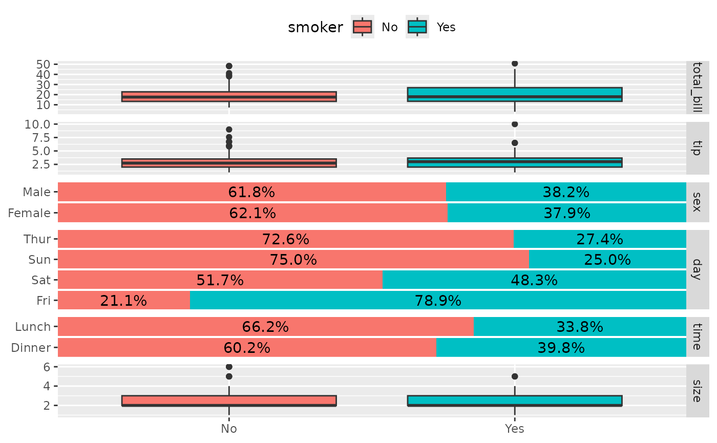
Column of six plots showing smoker status against total bill, tip, sex, day, time, and size, with the legend taken from the first sub-plot.

ggbivariate(tips, "smoker", legend = 3)
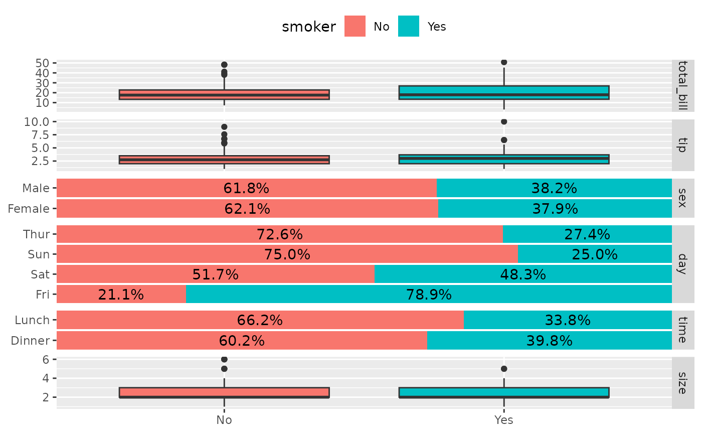
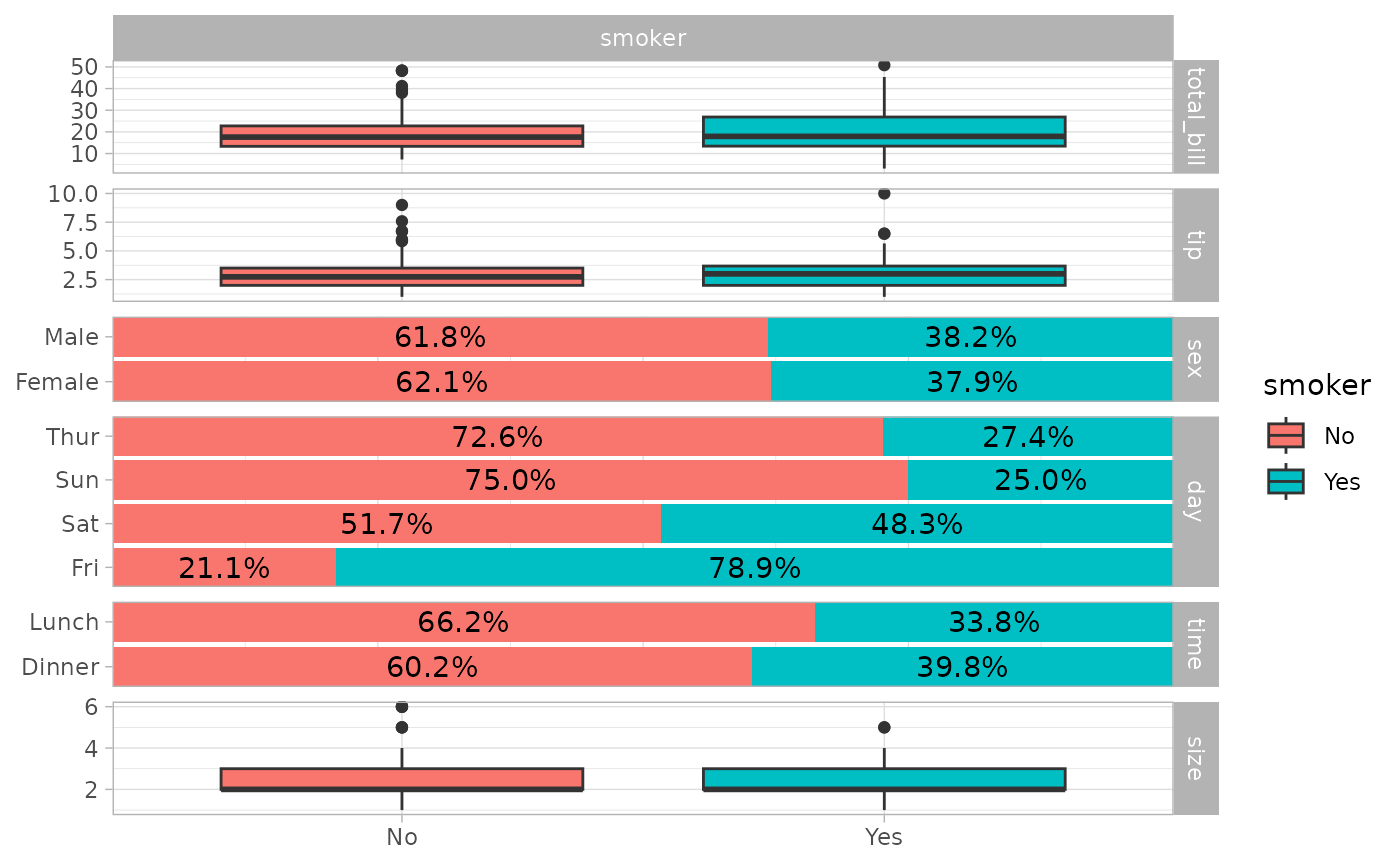
The same column of six plots showing smoker status against total bill, tip, sex, day, time, and size, with the legend taken from the third sub-plot.

Change theme

ggbivariate(tips, "smoker") + theme_light()

Column of six plots showing smoker status against total bill, tip, sex, day, time, and size, drawn with the light theme: white panels, grey borders, and grey strip labels.

Use mapping to indicate weights

d <- as.data.frame(Titanic)
ggbivariate(d, "Survived", mapping = aes(weight = Freq))
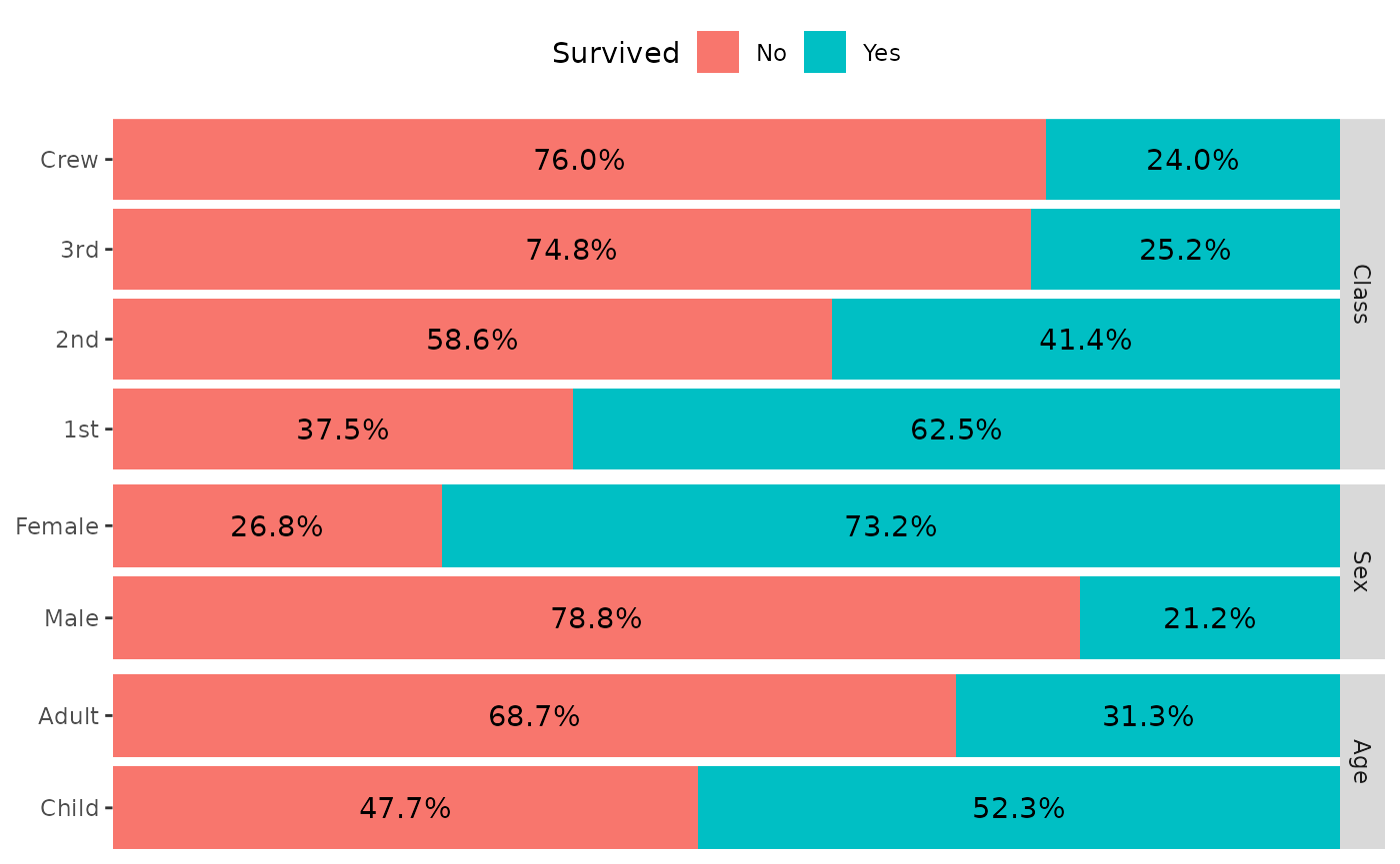
Column of three stacked percentage bar charts showing Titanic survival against class, sex, and age, weighted by passenger count. Survival is highest in first class, for women, and for children, and lowest for the crew and third class.

Use types to customize types of subplots

ggbivariate(
  tips,
  outcome = "smoker",
  explanatory = c("day", "time", "sex", "tip"),
  types = list(comboVertical = "autopoint")
)
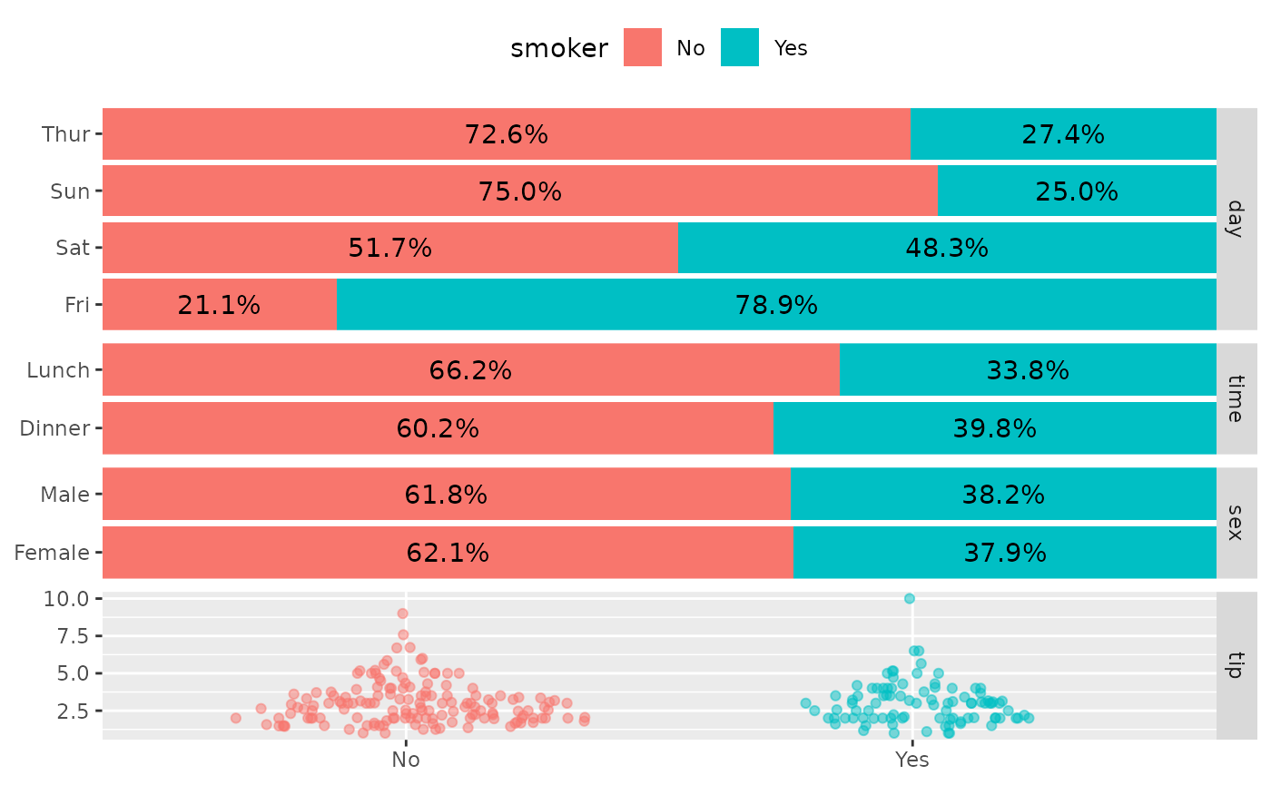
Column of four plots showing smoker status against day, time, sex, and tip. Day, time, and sex are stacked percentage bars, and tip is shown as jittered points for smokers and non-smokers instead of box plots.

For more customization options, you could directly use ggduo() (see also vig_ggally("ggduo")).