Skip to contents
library(GGally)
#> Loading required package: ggplot2

GGally::ggtable()

The purpose of this function is to quickly plot cross-tabulated tables of discrete variables.

Basic example

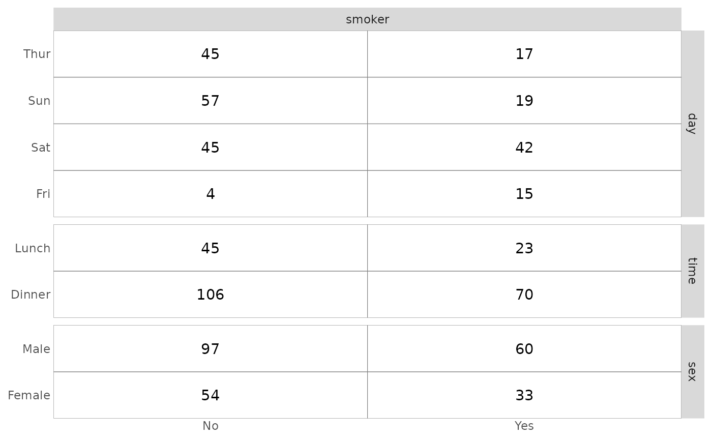
To display tables with the number of observations, simply indicate variables to present in columns and in rows.
data(tips)
ggtable(tips, "smoker", c("day", "time", "sex"))

Column of three cross-tabulated count tables, with smoker status across the top and day, time, and sex as the stacked rows. Each cell shows the number of tips.

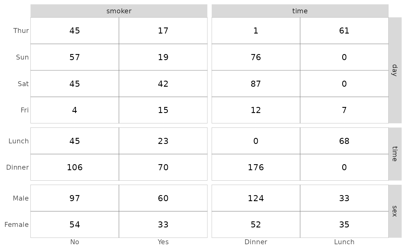
ggtable(tips, c("smoker", "time"), c("day", "time", "sex"))

Grid of cross-tabulated count tables with smoker status and time as the two columns and day, time, and sex as the three rows.

Proportions

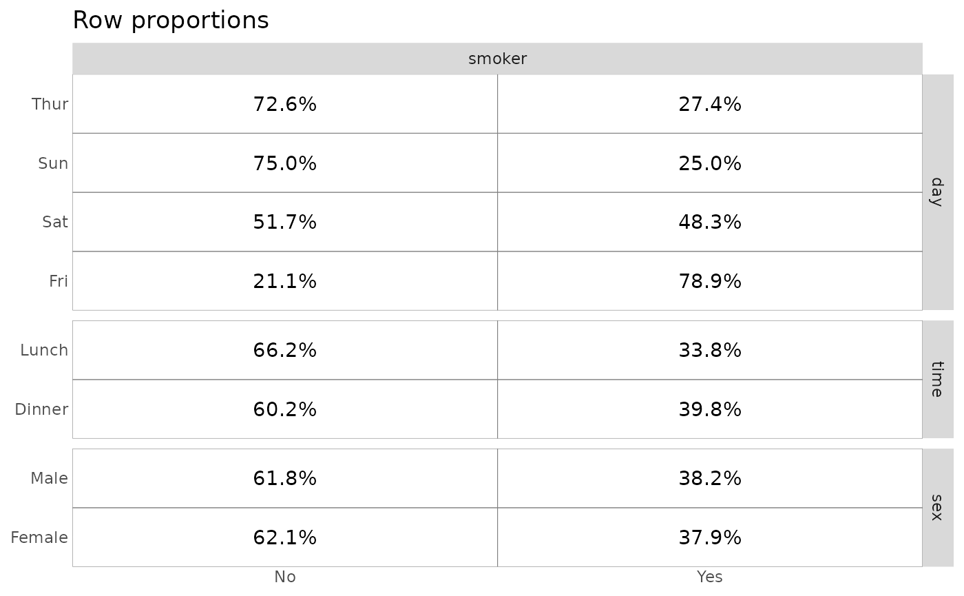
The cells argument allows you to control what to display. For proportions of the total, row proportions or columns proportions, simply use "prop", "row.prop" or "col.prop".
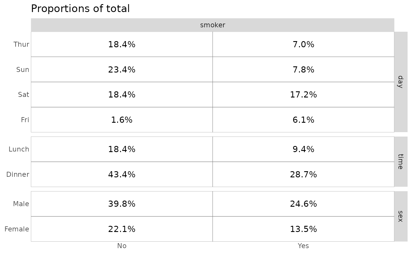
ggtable(tips, "smoker", c("day", "time", "sex"), cells = "prop") + ggtitle("Proportions of total")

Column of three cross-tabulated tables of smoker status by day, time, and sex, titled 'Proportions of total', with each cell showing its percentage of all tips.

ggtable(tips, "smoker", c("day", "time", "sex"), cells = "row.prop") + ggtitle("Row proportions")

Column of three cross-tabulated tables of smoker status by day, time, and sex, titled 'Row proportions', with each cell showing its percentage within its table row (one day, time, or sex).

ggtable(tips, "smoker", c("day", "time", "sex"), cells = "col.prop") + ggtitle("Column proportions")
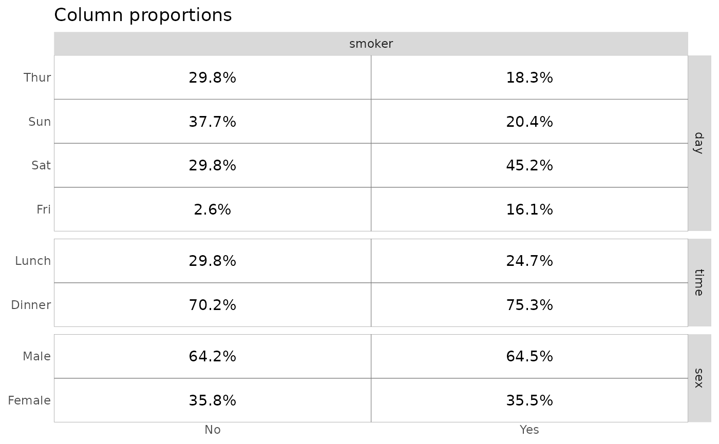
Column of three cross-tabulated tables of smoker status by day, time, and sex, titled 'Column proportions', with each cell showing its percentage within its smoker column.

Filling cells with residuals

Chi-square standardized residuals indicates which cells are over- or underrepresented compared to what would be expected under the independence hypothesis. If the standardized residual is less than -2, the cell’s observed frequency is less than the expected frequency. Greater than 2 and the observed frequency is greater than the expected frequency. Values lower than -3 or higher than 3 indicates a strong effect.

To fill cells with standardized residuals, simply indicate fill = "std.resid".
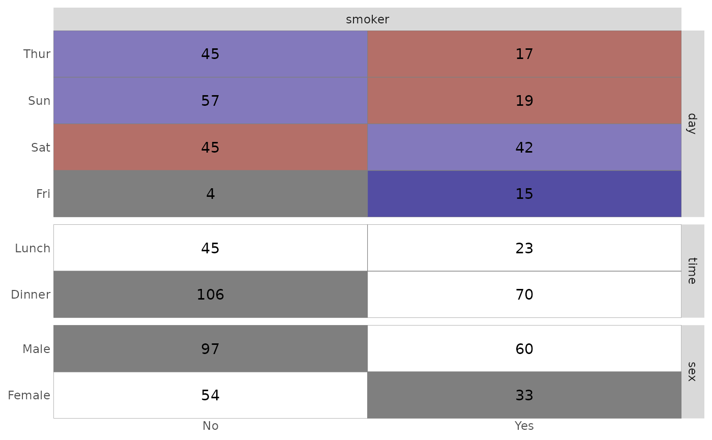
ggtable(tips, "smoker", c("day", "time", "sex"), fill = "std.resid")

Column of three cross-tabulated count tables of smoker status by day, time, and sex, with cells filled by standardized residual from red (fewer than expected) to blue (more than expected). Smokers are over-represented on Friday and Saturday and under-represented on Thursday and Sunday, while time and sex cells stay near zero.

Using weights

You can easily indicate weights to take into account with the weight aesthetic.

d <- as.data.frame(Titanic)
ggtable(
  d,
  "Survived",
  c("Age", "Class", "Sex"),
  mapping = aes(weight = Freq),
  cells = "row.prop",
  fill = "std.resid"
)
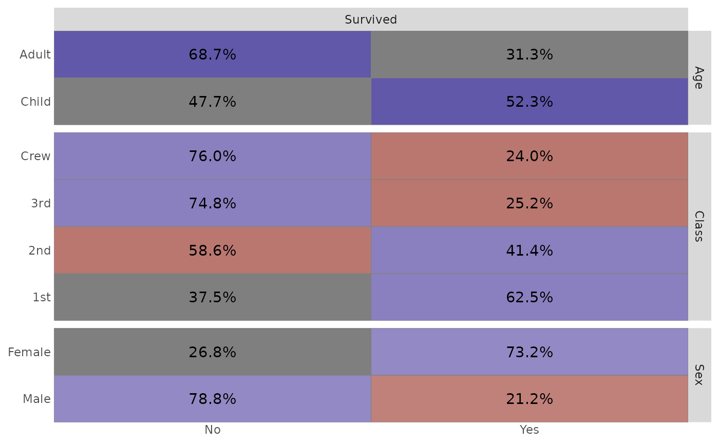
Column of three cross-tabulated tables of Titanic survival by age, class, and sex, showing row percentages weighted by passenger count and filled by standardized residual. Survivors are strongly over-represented among women, children, and first class, and under-represented among men, the crew, and third class.

Missing with continuous variables

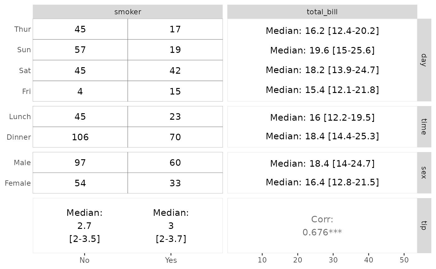
Although ggtable() is mainly intended to be used with discrete variables, you can also indicate continuous variables. In such case, some summary statistics are displayed.

ggtable(tips, c("smoker", "total_bill"), c("day", "time", "sex", "tip"))

Grid of panels with smoker status and total bill as the columns and day, time, sex, and tip as the rows. Discrete pairs show count tables, and pairs with a continuous variable show summary statistics as text.

If you need more customization of the output, please refer to ggduo().