glyphs(): Glyph plot
Hadley Wickham, Charlotte Wickham, Di Cook, Heike Hofmann
Nov 6, 2015
Source:vignettes/glyph.Rmd
glyph.Rmd
GGally::glyphs()
This function rearranges data to be able to construct a glyph plot
library(ggplot2)
data(nasa)
temp.gly <- glyphs(nasa, "long", "day", "lat", "surftemp", height = 2.5)
#> Using width 2.38
ggplot(temp.gly, ggplot2::aes(gx, gy, group = gid)) +
  add_ref_lines(temp.gly, color = "grey90") +
  add_ref_boxes(temp.gly, color = "grey90") +
  geom_path() +
  theme_bw() +
  labs(x = "", y = "")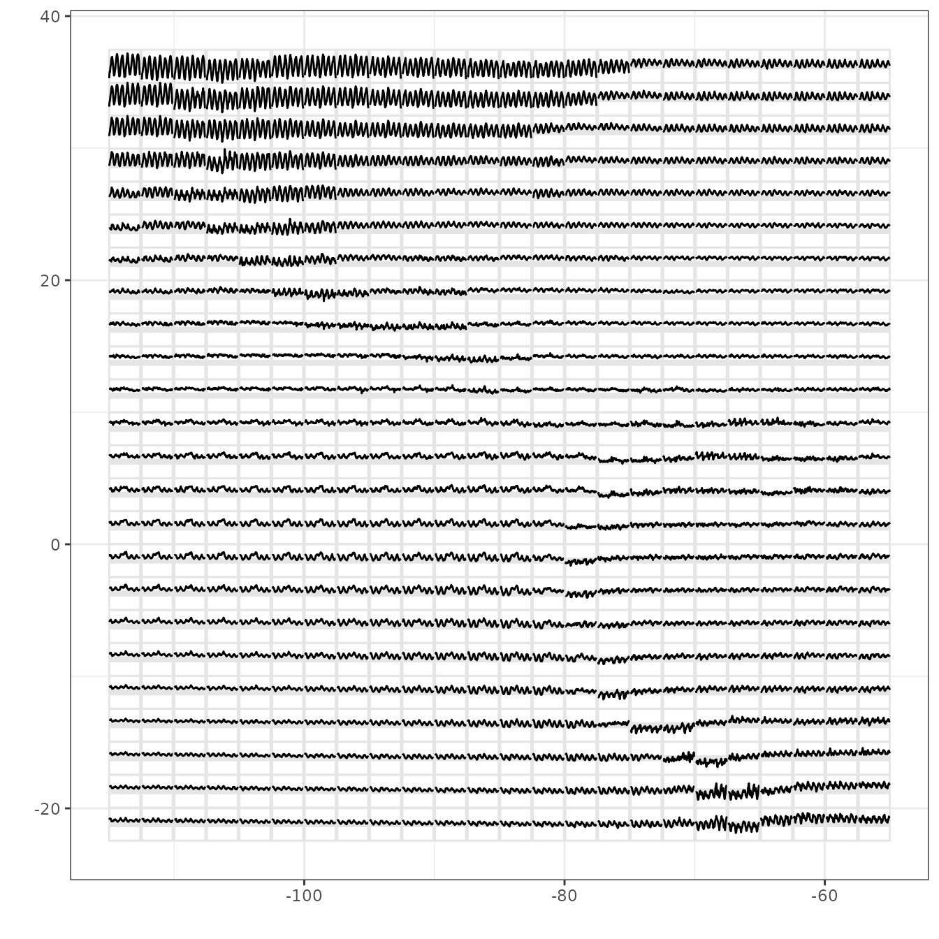
This shows a glyphplot of monthly surface temperature for 6 years over Central America. You can see differences from one location to another, that in large areas temperature doesn’t change much. There are large seasonal trends in the top left over land.
Rescaling in different ways puts emphasis on different components, see the examples in the referenced paper. And with ggplot2 you can make a map of the geographic area underlying the glyphs.