ggnetworkmap(): Network + map plot
Amos Elberg
Jan 10, 2015
Source:vignettes/ggnetworkmap.Rmd
ggnetworkmap.Rmd
GGally::ggnetworkmap()
ggnetworkmap() is a function for plotting elegant maps
using ggplot2. It builds on ggnet() by
allowing to draw a network over a map, and is particularly intended for
use with ggmap.
Example: US airports
This example is based on a tutorial
by Nathan Yau at Flowing Data. The airport locations come from the
FAA data in airports::usairports.
suppressMessages(library(ggplot2))
suppressMessages(library(maps))
suppressMessages(library(network))
suppressMessages(library(sna))

# convert "DD-MM-SS.SSSSN" coordinates to decimal degrees
dms_to_number <- function(dms) {
  parts <- strsplit(dms, "-")[[1]]
  degrees <- as.numeric(parts[1])
  minutes <- as.numeric(parts[2]) / 60
  seconds <- as.numeric(sub(parts[3], pattern = "N|W", replacement = "")) / 3600
  direction <- if (grepl("W", parts[3])) -1 else 1
  direction * (degrees + minutes + seconds)
}

# keep certified airports in the northern and western hemispheres
airports <- as.data.frame(airports::usairports)
airports <- subset(
  airports,
  !is.na(cert_type_date) & grepl("N", arp_latitude) & grepl("W", arp_longitude)
)
airports$lat <- vapply(airports$arp_latitude, dms_to_number, numeric(1))
airports$long <- vapply(airports$arp_longitude, dms_to_number, numeric(1))
rownames(airports) <- airports$location_id

# select some random flights
set.seed(123)
flights <- data.frame(
  origin = sample(airports[200:400, ]$location_id, 200, replace = TRUE),
  destination = sample(airports[200:400, ]$location_id, 200, replace = TRUE)
)

# convert to network
flights <- network(flights, directed = TRUE)

# add geographic coordinates
flights %v% "lat" <- airports[network.vertex.names(flights), "lat"]
flights %v% "lon" <- airports[network.vertex.names(flights), "long"]

# drop isolated airports
delete.vertices(flights, which(degree(flights) < 2))

# compute degree centrality
flights %v% "degree" <- degree(flights, gmode = "digraph")

# add random groups
flights %v% "mygroup" <- sample(letters[1:4], network.size(flights), replace = TRUE)

# create a map of the USA
usa <- ggplot(map_data("usa"), aes(x = long, y = lat)) +
  geom_polygon(aes(group = group),
    color = "grey65",
    fill = "#f9f9f9", linewidth = 0.2
  )

# trim flights
delete.vertices(flights, which(flights %v% "lon" < min(usa$data$long)))
delete.vertices(flights, which(flights %v% "lon" > max(usa$data$long)))
delete.vertices(flights, which(flights %v% "lat" < min(usa$data$lat)))
delete.vertices(flights, which(flights %v% "lat" > max(usa$data$lat)))

# overlay network data to map
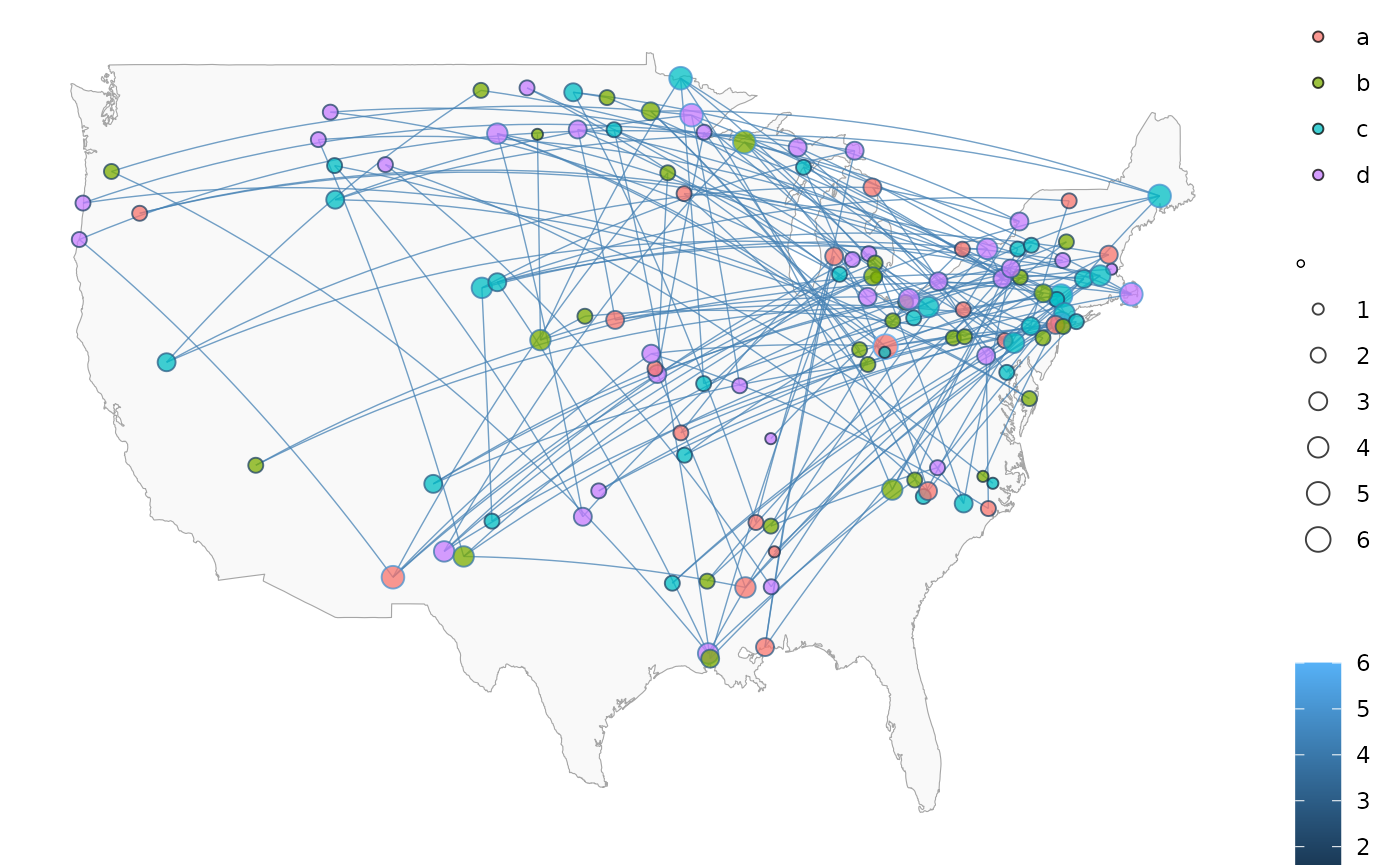
ggnetworkmap(usa, flights,
  size = 4, great.circles = TRUE,
  node.group = mygroup, segment.color = "steelblue",
  ring.group = degree, weight = degree
)
Example: Twitter spambots
This next example uses data from a Twitter spam community identified while exploring and trying to clear-up a group of tweets. After coloring the nodes based on their centrality, the odd structure stood out clearly.
data(twitter_spambots)
# create a world map
world <- fortify(map("world", plot = FALSE, fill = TRUE))
#> Warning: `fortify(<map>)` was deprecated in ggplot2 4.0.0.
#> ℹ Please use `map_data()` instead.
#> This warning is displayed once per session.
#> Call `lifecycle::last_lifecycle_warnings()` to see where this warning was
#> generated.
world <- ggplot(world, aes(x = long, y = lat)) +
  geom_polygon(aes(group = group),
    color = "grey65",
    fill = "#f9f9f9", linewidth = 0.2
  )

# view global structure
ggnetworkmap(world, twitter_spambots)
#> Ignoring unknown labels:
#> • colour : ""
#> • fill : ""
#> • size : ""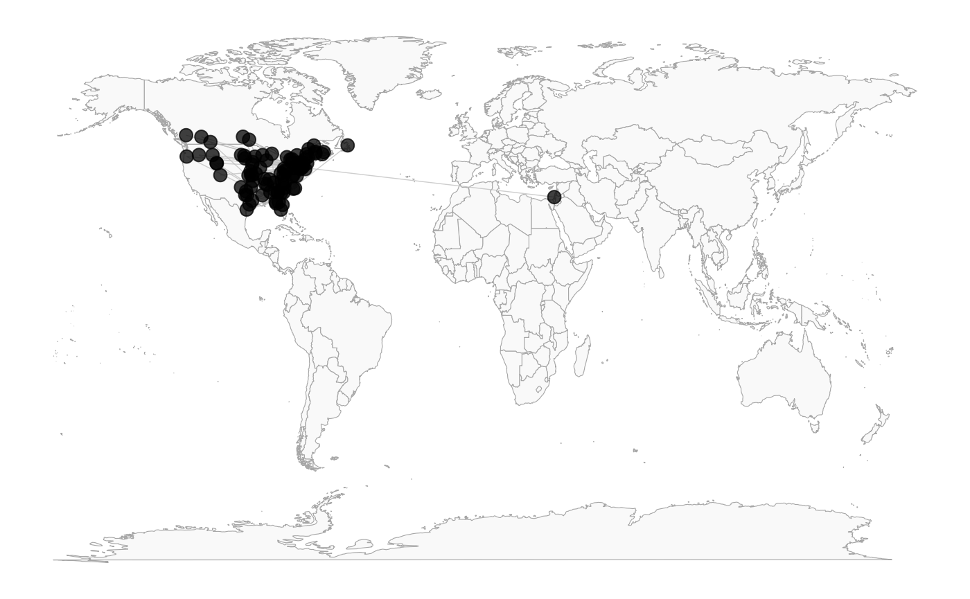
Is the network really concentrated in the U.S.? Probably not. One of the odd things about the network, is a much higher proportion of the users gave locations that could be geocoded, than Twitter users generally.
Let’s see the network topology
ggnetworkmap(net = twitter_spambots, arrow.size = 0.5)
#> Ignoring unknown labels:
#> • colour : ""
#> • fill : ""
#> • size : ""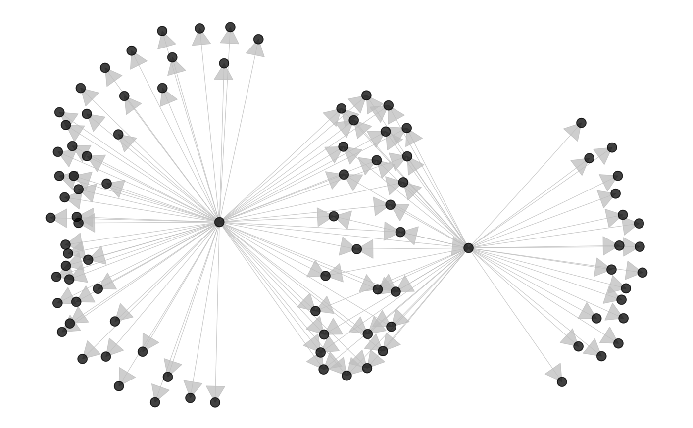
Coloring nodes according to degree centrality can highlight network structures.
# compute indegree and outdegree centrality
twitter_spambots %v% "indegree" <- degree(twitter_spambots, cmode = "indegree")
twitter_spambots %v% "outdegree" <- degree(twitter_spambots, cmode = "outdegree")

ggnetworkmap(
  net = twitter_spambots,
  arrow.size = 0.5,
  node.group = indegree,
  ring.group = outdegree, size = 4
) +
  scale_fill_continuous("Indegree", high = "red", low = "yellow") +
  labs(color = "Outdegree")
#> Ignoring unknown labels:
#> • size : ""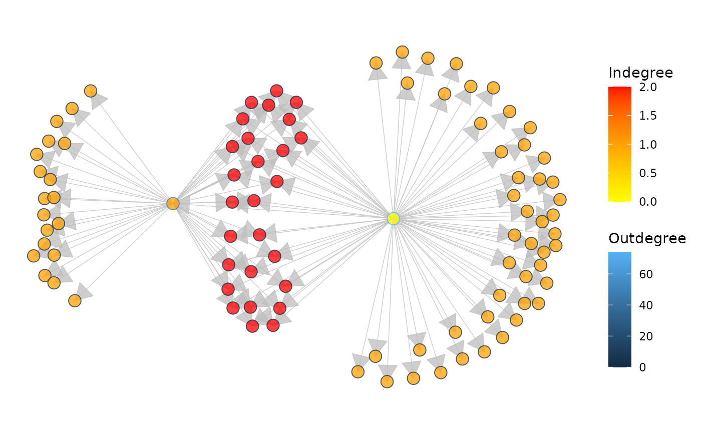
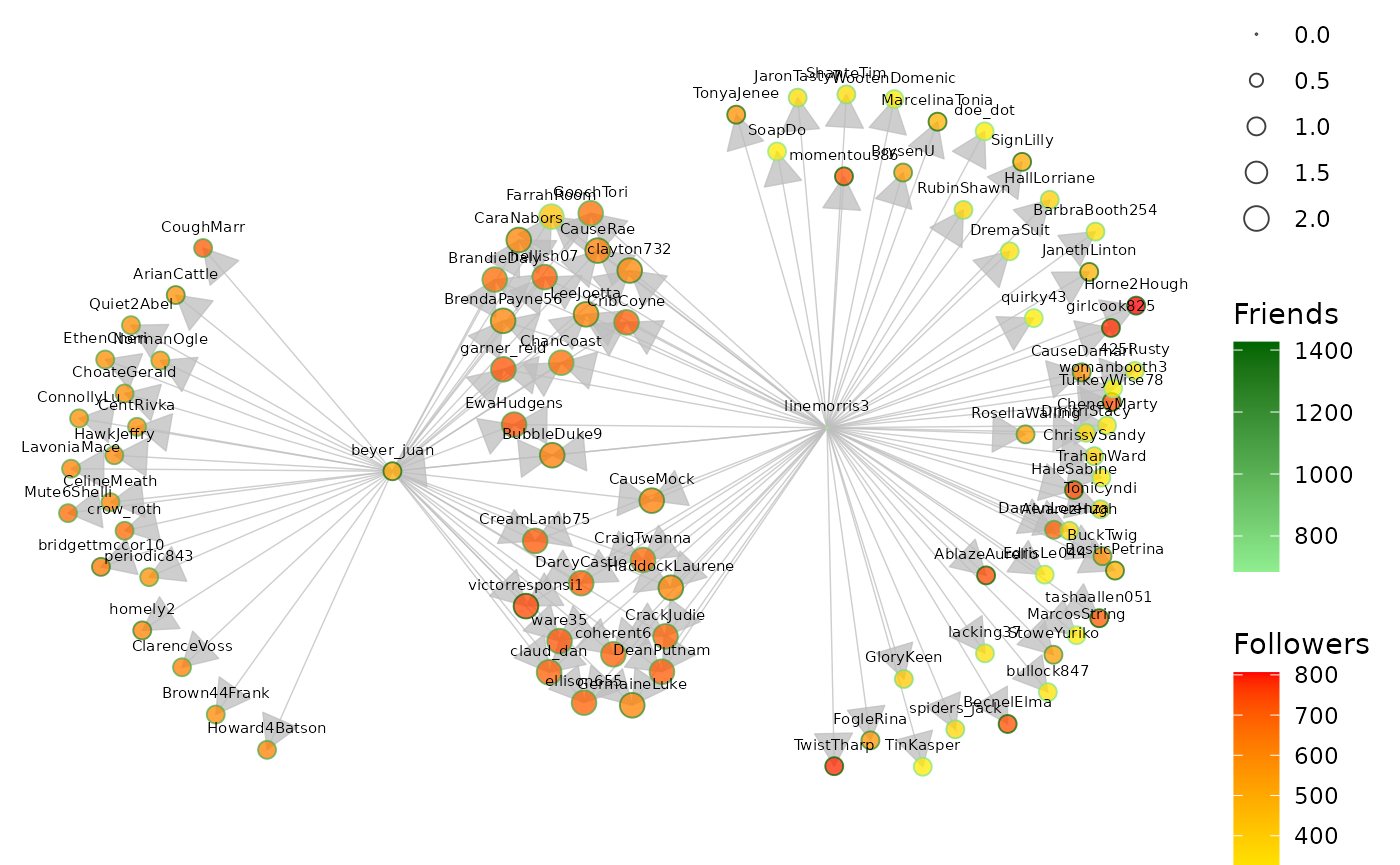
Some Twitter attributes have been included as vertex attributes.
# show some vertex attributes associated with each account
ggnetworkmap(
  net = twitter_spambots,
  arrow.size = 0.5,
  node.group = followers,
  ring.group = friends,
  size = 4,
  weight = indegree,
  label.nodes = TRUE, vjust = -1.5
) +
  scale_fill_continuous("Followers", high = "red", low = "yellow") +
  labs(color = "Friends") +
  scale_color_continuous(low = "lightgreen", high = "darkgreen")