ggduo(): Two-grouped plot matrix
Barret Schloerke
July 4, 2016
Source:vignettes/ggduo.Rmd
ggduo.Rmd
GGally::ggduo()
The purpose of this function is to display two grouped data in a plot matrix. This is useful for canonical correlation analysis, multiple time series analysis, and regression analysis.
Canonical Correlation Analysis
This example is derived from
R Data Analysis Examples | Canonical Correlation Analysis. UCLA: Institute for Digital Research and Education. from http://www.stats.idre.ucla.edu/r/dae/canonical-correlation-analysis (accessed May 22, 2017).
Example 1. A researcher has collected data on three psychological variables, four academic variables (standardized test scores) and gender for 600 college freshman. She is interested in how the set of psychological variables relates to the academic variables and gender. In particular, the researcher is interested in how many dimensions (canonical variables) are necessary to understand the association between the two sets of variables."
data(psychademic)
str(psychademic)
#> 'data.frame':    600 obs. of  8 variables:
#>  $ locus_of_control: num  -0.84 -0.38 0.89 0.71 -0.64 1.11 0.06 -0.91 0.45 0 ...
#>  $ self_concept    : num  -0.24 -0.47 0.59 0.28 0.03 0.9 0.03 -0.59 0.03 0.03 ...
#>  $ motivation      : chr  "4" "3" "3" "3" ...
#>  $ read            : num  54.8 62.7 60.6 62.7 41.6 62.7 41.6 44.2 62.7 62.7 ...
#>  $ write           : num  64.5 43.7 56.7 56.7 46.3 64.5 39.1 39.1 51.5 64.5 ...
#>  $ math            : num  44.5 44.7 70.5 54.7 38.4 61.4 56.3 46.3 54.4 38.3 ...
#>  $ science         : num  52.6 52.6 58 58 36.3 58 45 36.3 49.8 55.8 ...
#>  $ sex             : chr  "female" "female" "male" "male" ...
#>  - attr(*, "academic")= chr [1:5] "read" "write" "math" "science" ...
#>  - attr(*, "psychology")= chr [1:3] "locus_of_control" "self_concept" "motivation"
(psych_variables <- attr(psychademic, "psychology"))
#> [1] "locus_of_control" "self_concept"     "motivation"
(academic_variables <- attr(psychademic, "academic"))
#> [1] "read"    "write"   "math"    "science" "sex"
First, look at the within correlation using
ggpairs().
ggpairs(psychademic, psych_variables, title = "Within Psychological Variables")
#> `stat_bin()` using `bins = 30`. Pick better value `binwidth`.
#> `stat_bin()` using `bins = 30`. Pick better value `binwidth`.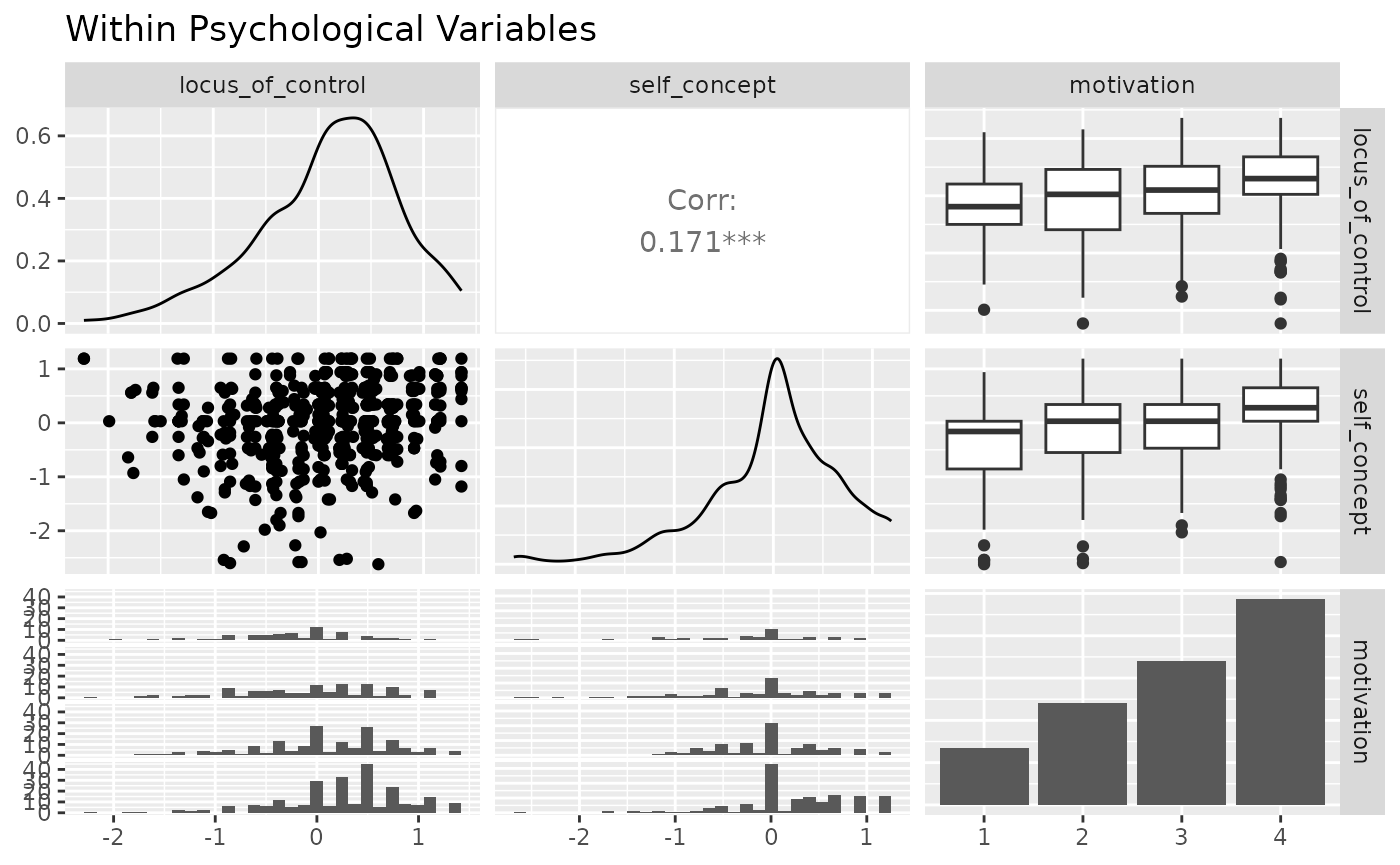
ggpairs(psychademic, academic_variables, title = "Within Academic Variables")
#> `stat_bin()` using `bins = 30`. Pick better value `binwidth`.
#> `stat_bin()` using `bins = 30`. Pick better value `binwidth`.
#> `stat_bin()` using `bins = 30`. Pick better value `binwidth`.
#> `stat_bin()` using `bins = 30`. Pick better value `binwidth`.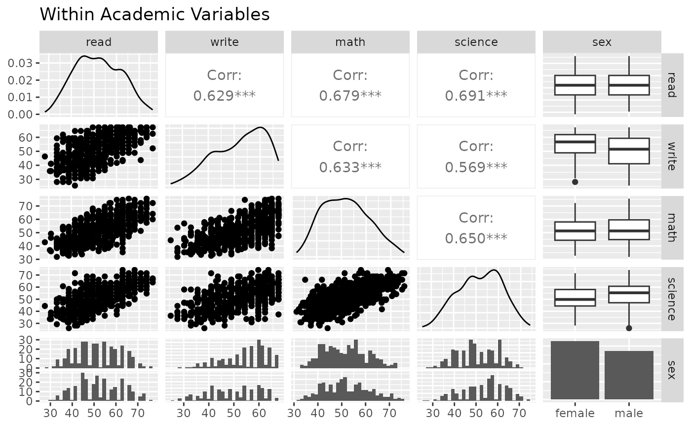
Next, look at the between correlation using ggduo().
ggduo(
  psychademic, psych_variables, academic_variables,
  types = list(continuous = "smooth_lm"),
  title = "Between Academic and Psychological Variable Correlation",
  xlab = "Psychological",
  ylab = "Academic"
)
#> `stat_bin()` using `bins = 30`. Pick better value `binwidth`.
#> `stat_bin()` using `bins = 30`. Pick better value `binwidth`.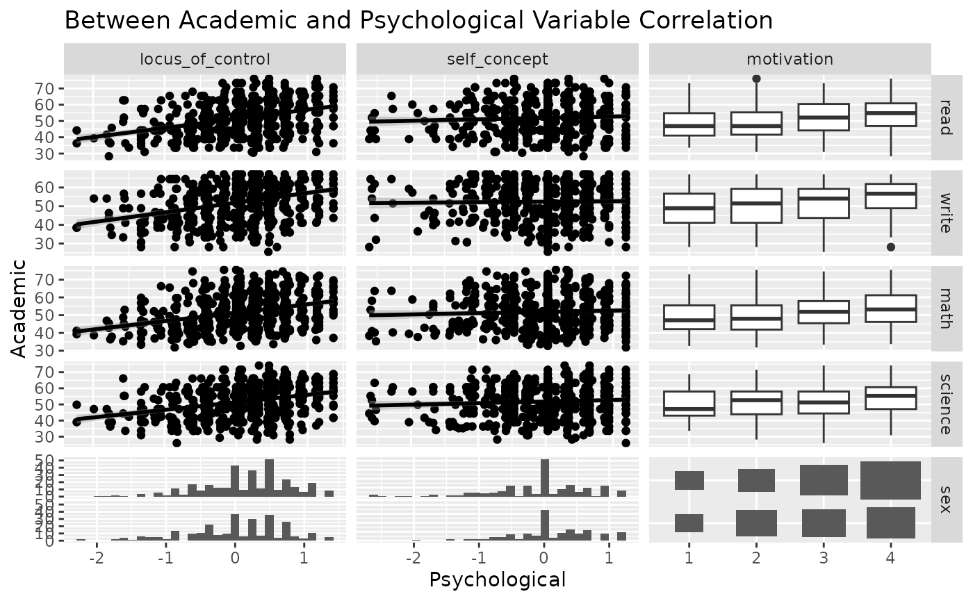
Since ggduo does not have a upper section to display the correlation values, we may use a custom function to add the information in the continuous plots. The strips may be removed as each group name may be recovered in the outer axis labels.
lm_with_cor <- function(data, mapping, ..., method = "pearson") {
  x <- eval_data_col(data, mapping$x)
  y <- eval_data_col(data, mapping$y)
  cor <- cor(x, y, method = method)
  ggally_smooth_lm(data, mapping, ...) +
    ggplot2::geom_label(
      data = data.frame(
        x = min(x, na.rm = TRUE),
        y = max(y, na.rm = TRUE),
        lab = round(cor, digits = 3)
      ),
      mapping = ggplot2::aes(x = x, y = y, label = lab),
      hjust = 0, vjust = 1,
      size = 5, fontface = "bold",
      inherit.aes = FALSE # do not inherit anything from the ...
    )
}
ggduo(
  psychademic, rev(psych_variables), academic_variables,
  mapping = aes(color = sex),
  types = list(continuous = wrap(lm_with_cor, alpha = 0.25)),
  showStrips = FALSE,
  title = "Between Academic and Psychological Variable Correlation",
  xlab = "Psychological",
  ylab = "Academic",
  legend = c(5, 2)
) +
  theme(legend.position = "bottom")
#> `stat_bin()` using `bins = 30`. Pick better value `binwidth`.
#> `stat_bin()` using `bins = 30`. Pick better value `binwidth`.
#> `stat_bin()` using `bins = 30`. Pick better value `binwidth`.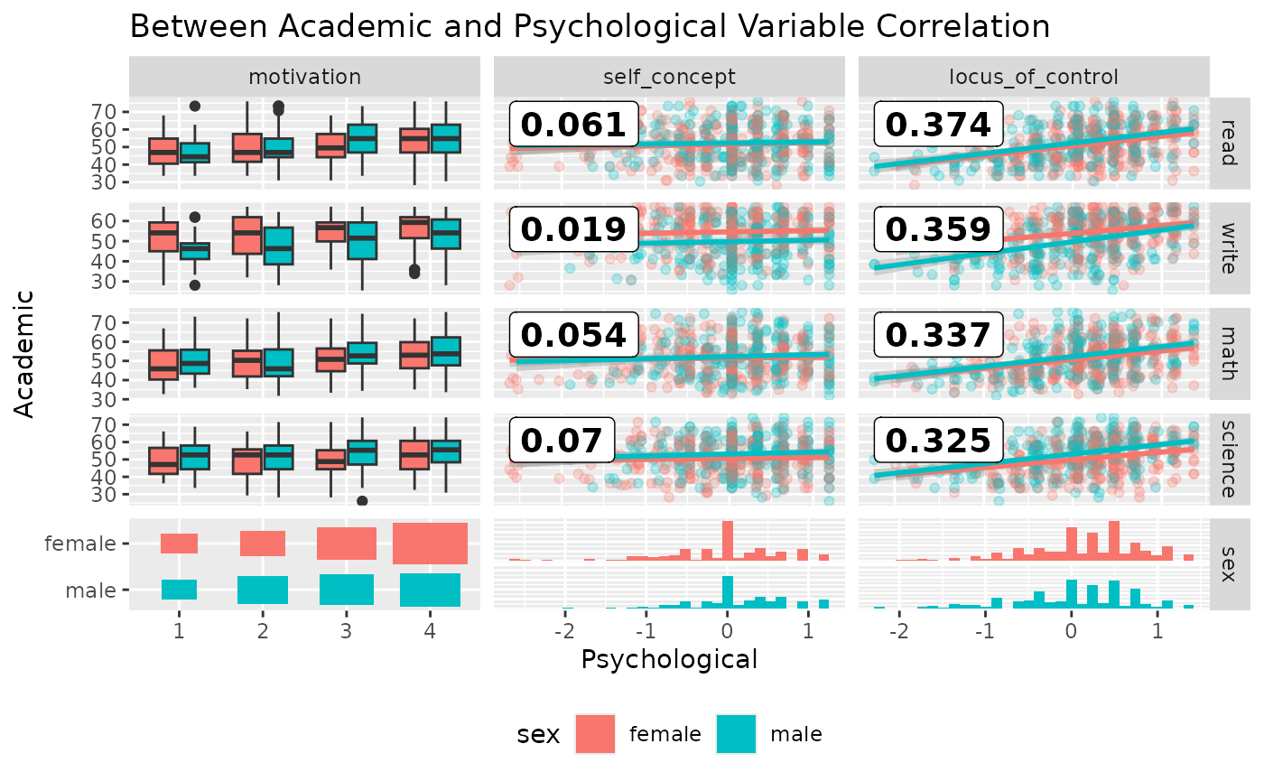
Multiple Time Series Analysis
While displaying multiple time series vertically over time, such as
+ ggplot2::facet_grid(time ~ .), ggduo() can
handle both continuous and discrete data. ggplot2 does not
mix discrete and continuous data on the same axis.
library(ggplot2)

data(pigs)
pigs_dt <- pigs[-(2:3)] # remove year and quarter
pigs_dt$profit_group <- as.numeric(pigs_dt$profit > mean(pigs_dt$profit))
ggplot(
  tidyr::pivot_longer(pigs_dt, -time),
  aes(x = time, y = value)
) +
  geom_smooth() +
  geom_point() +
  facet_grid(name ~ ., scales = "free_y")
#> `geom_smooth()` using method = 'loess' and formula = 'y ~ x'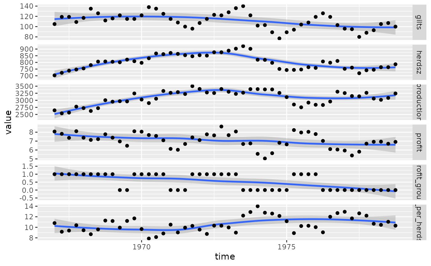
Instead, we may use ggts to display the data.
ggts changes the default behavior of ggduo of
columnLabelsX to equal NULL and allows for
mixed variable types.
# make the profit group as a factor value
profit_groups <- c(
  "1" = "high",
  "0" = "low"
)
pigs_dt$profit_group <- factor(
  profit_groups[as.character(pigs_dt$profit_group)],
  levels = unname(profit_groups),
  ordered = TRUE
)
ggts(pigs_dt, "time", 2:7)
#> `stat_bin()` using `bins = 30`. Pick better value `binwidth`.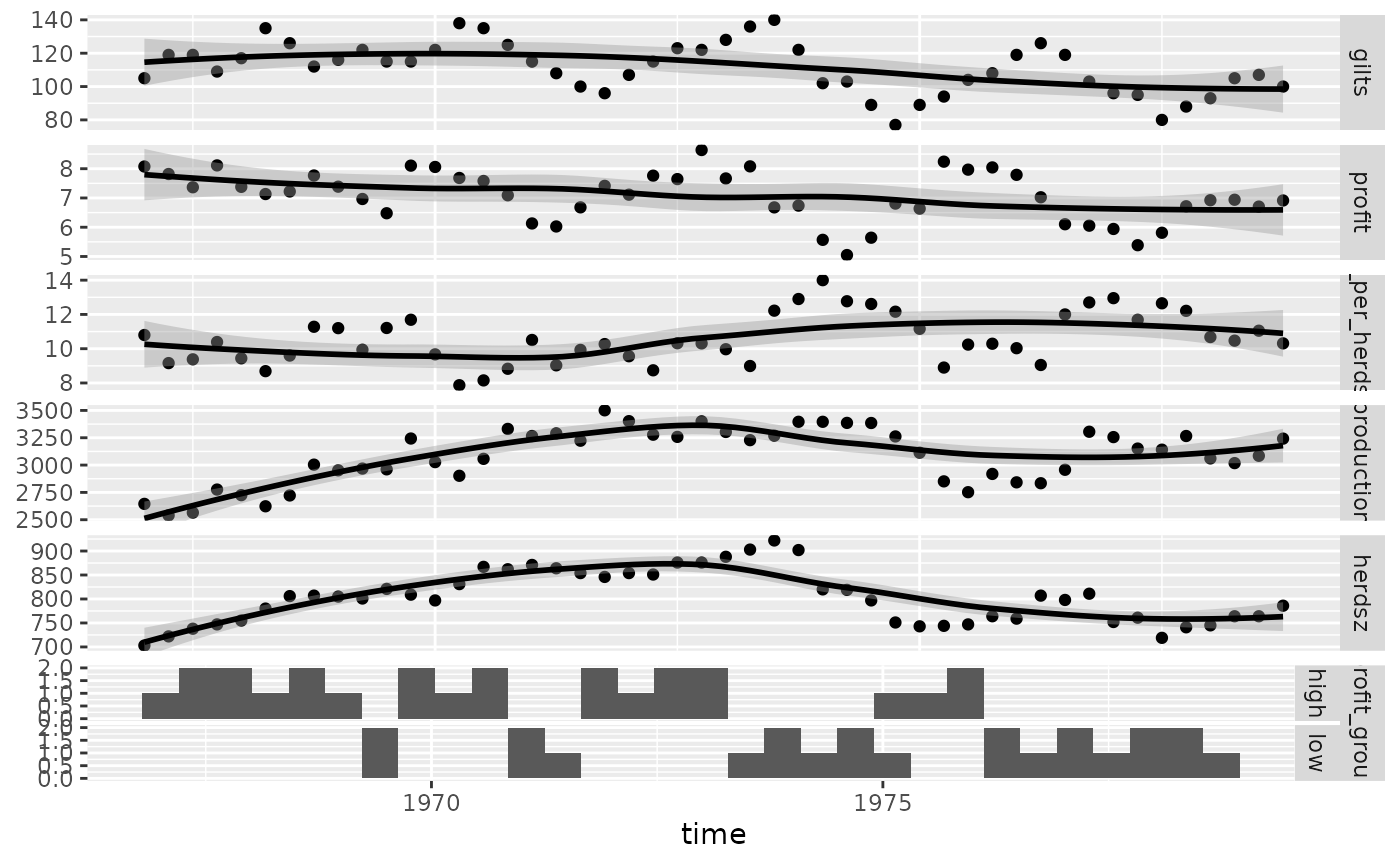
# remove the binwidth warning
pigs_types <- list(
  comboHorizontal = wrap(ggally_facethist, binwidth = 1)
)
ggts(pigs_dt, "time", 2:7, types = pigs_types)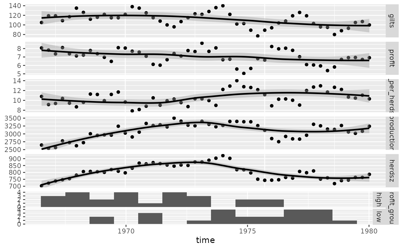
# add color and legend
pigs_mapping <- aes(color = profit_group)
ggts(pigs_dt, pigs_mapping, "time", 2:7, types = pigs_types, legend = c(6, 1))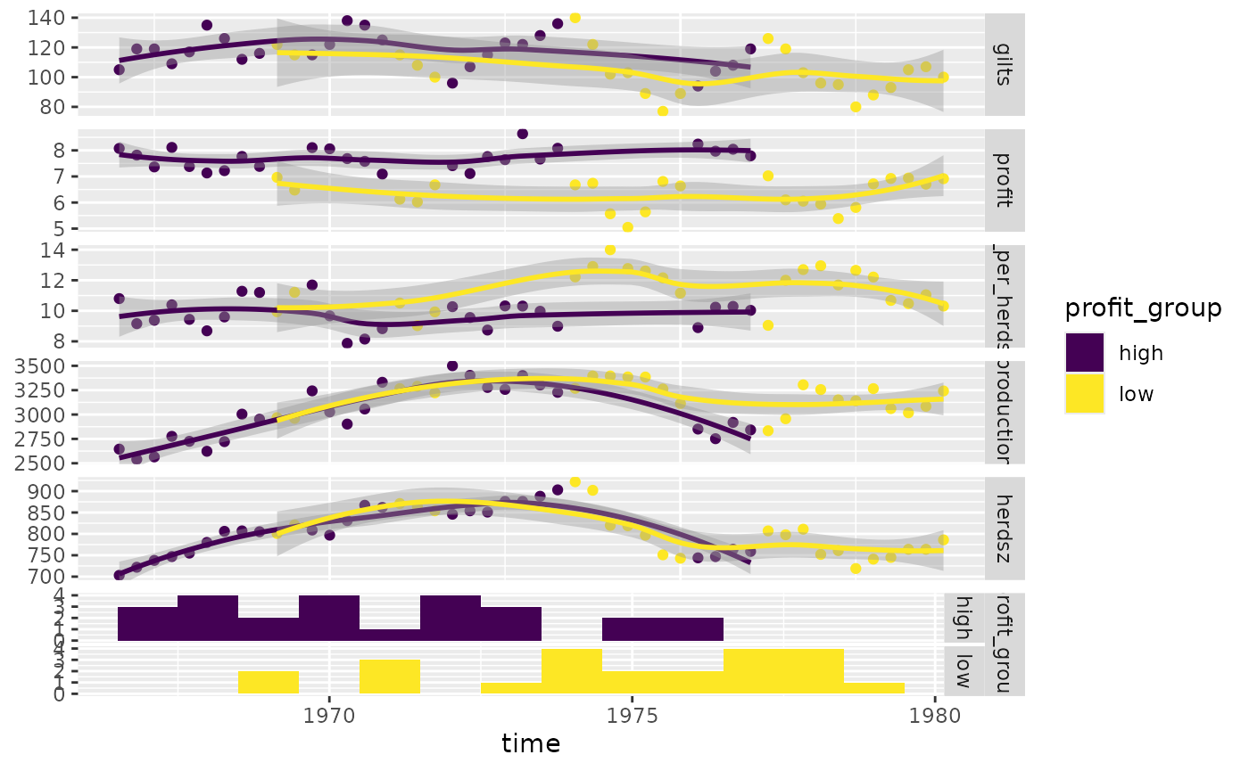
Produce more meaningful labels, add a legend, and remove profit group strips.
pm <- ggts(
  pigs_dt, pigs_mapping,
  1, 2:7,
  types = pigs_types,
  legend = c(6, 1),
  columnLabelsY = c(
    "number of\nfirst birth sows",
    "sell price over\nfeed cost",
    "sell count over\nheard size",
    "meat head count",
    "breading\nheard size",
    "profit\ngroup"
  ),
  showStrips = FALSE
) +
  labs(fill = "profit group") +
  theme(
    legend.position = "bottom",
    strip.background = element_rect(
      fill = "transparent", color = "grey80"
    )
  )
pm
#> Ignoring unknown labels:
#> • fill : "profit group"
#> Ignoring unknown labels:
#> • fill : "profit group"
#> Ignoring unknown labels:
#> • fill : "profit group"
#> Ignoring unknown labels:
#> • fill : "profit group"
#> Ignoring unknown labels:
#> • fill : "profit group"
#> Ignoring unknown labels:
#> • fill : "profit group"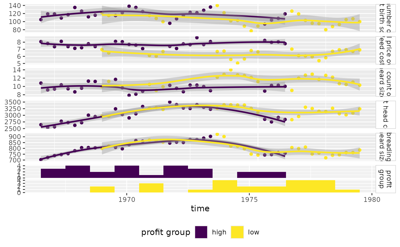
Regression Analysis
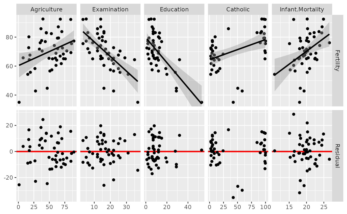
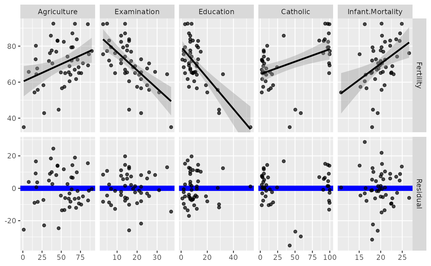
Since ggduo() may take custom functions just like
ggpairs(), we will make a custom function that displays the
residuals with a red line at 0 and all other y variables will receive a
simple linear regression plot.
Note: the marginal residuals are calculated before plotting and the y_range is found to display all residuals on the same scale.
swiss <- datasets::swiss

# add a 'fake' column
swiss$Residual <- seq_len(nrow(swiss))

# calculate all residuals prior to display
residuals <- lapply(swiss[2:6], function(x) {
  summary(lm(Fertility ~ x, data = swiss))$residuals
})
# calculate a consistent y range for all residuals
y_range <- range(unlist(residuals))

# custom function to display continuous data. If the y variable is "Residual", do custom work.
lm_or_resid <- function(data, mapping, ..., line_color = "red", line_size = 1) {
  if (!identical(
    rlang::expr_text(mapping$y),
    rlang::expr_text(ggplot2::aes(y = Residual)$y)
  )) {
    return(ggally_smooth_lm(data, mapping, ...))
  }

  # make residual data to display
  resid_data <- data.frame(
    x = rlang::eval_tidy(mapping$x, data = data),
    y = rlang::eval_tidy(mapping$x, data = residuals)
  )

  ggplot(data = data, mapping = mapping) +
    geom_hline(yintercept = 0, color = line_color, linewidth = line_size) +
    ylim(y_range) +
    geom_point(data = resid_data, mapping = aes(x = x, y = y), ...)
}

# plot the data
ggduo(
  swiss,
  2:6, c(1, 7),
  types = list(continuous = lm_or_resid)
)
# change line to be thicker and blue and the points to be slightly transparent
ggduo(
  swiss,
  2:6, c(1, 7),
  types = list(
    continuous = wrap(lm_or_resid,
      alpha = 0.7,
      line_color = "blue",
      line_size = 3
    )
  )
)
Types of plots
You can customize the type of plots to display with the
types argument. types is a list that may
contain the variables ‘continuous’, ‘combo’, ‘discrete’, and ‘na’. Each
element of the list may be a function or a string. If a string is
supplied, it must be a character string representing the tail end of a
ggally_NAME function.
-
continuous: when both x and y variables are continuous -
comboHorizontal: when x is continuous and y is discrete -
comboVorizontal: when x is discrete and y is continuous -
discrete: when both x and y variables are discrete -
na: when all x data and all y data isNA
The list of current valid ggally_NAME functions is
visible in vig_ggally("ggally_plots").