Working with legends

Stefan McKinnon Edwards sme@iysik.com

2025-09-17

Legend functions

• Extract legend: g_legend
• Reposition legend onto the actual plot: reposition_legend
• Combine multiple plots, but use only one legend: grid_arrange_shared_legend

Reposition legend onto plotting panel

ggplot2 by default places the legend in the margin of the entire plot. This is in many instances a nice solution. If this is not desired, theme(legend.position) can be used to place the legend in relative measures on the entire plot:

library(ggplot2)
library(grid)
library(gridExtra)
dsamp <- diamonds[sample(nrow(diamonds), 1000), ]
(d <- ggplot(dsamp, aes(carat, price)) +
  geom_point(aes(colour = clarity)) +
  theme(legend.position = c(0.06, 0.75))
)

Imprecise positioning of legend with theme(legend.position).

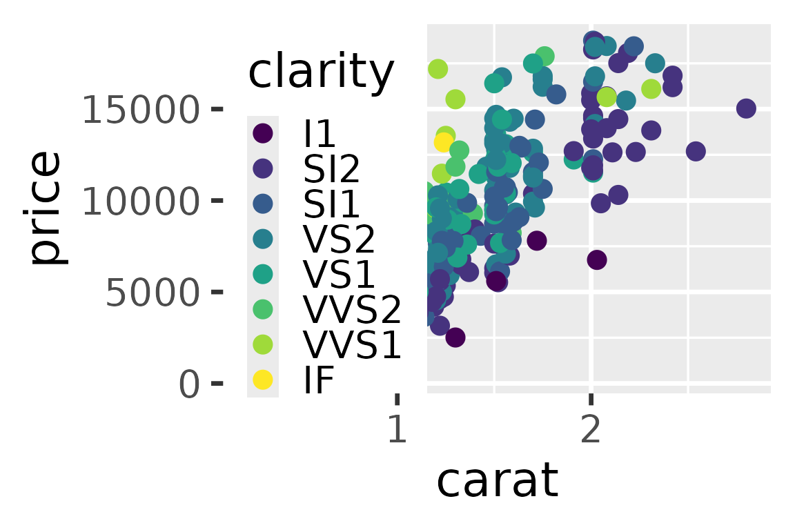
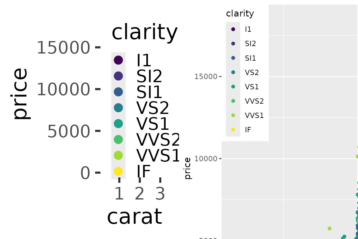
This is however prone to badly positioning, if e.g. the plot is resized or font size changed:

Left: Base font size set to 22 pt. Right: Zoom on plot that is plotted at 150% size.

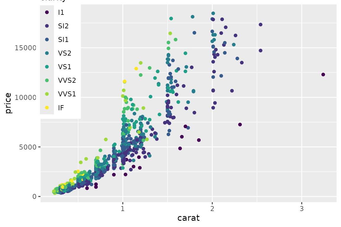
With our function, we can specify exactly how we want it in the plotting area:

library(lemon)
reposition_legend(d, 'top left')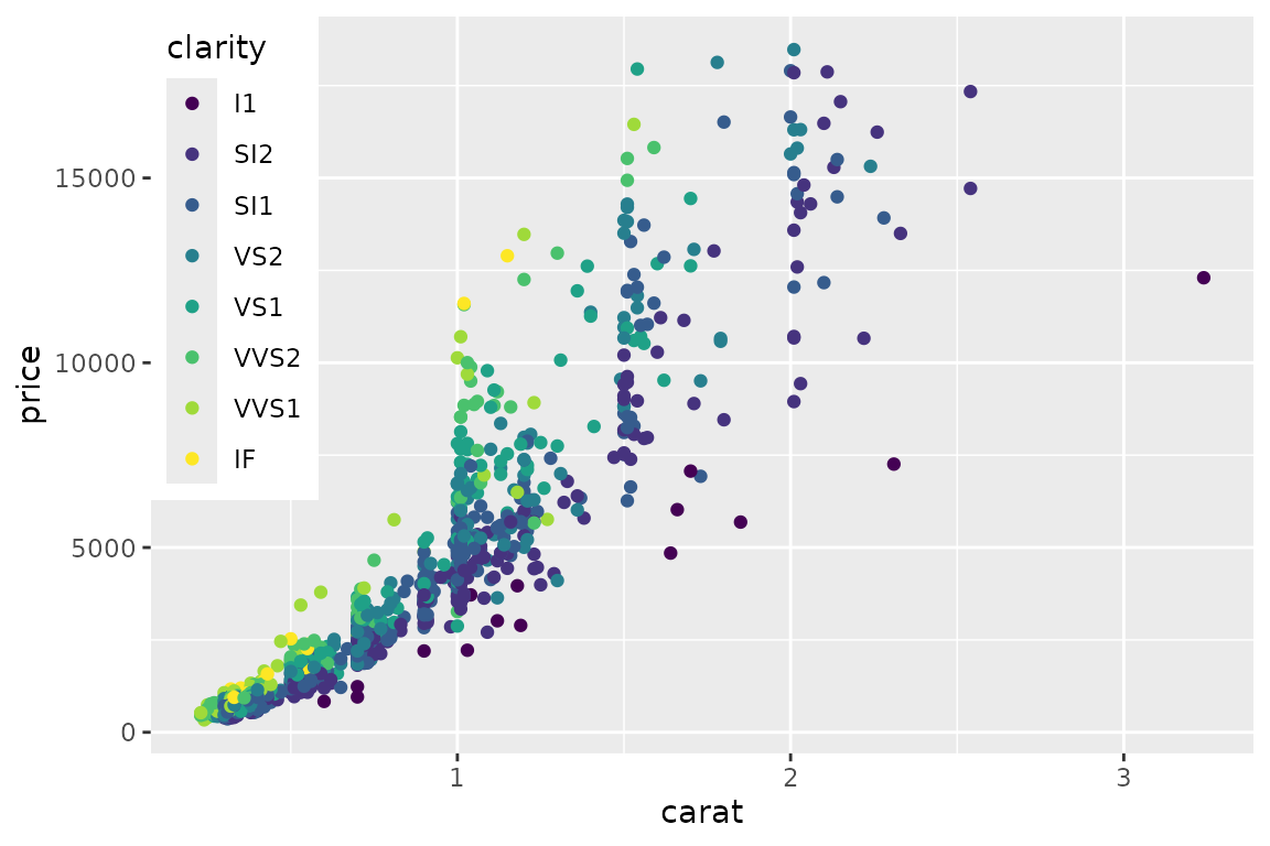

Exact positioning of legend in the main panel.

And it stays there.

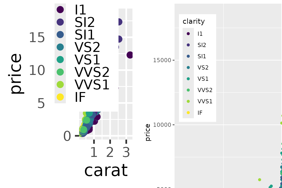
Left: Base font size set to 22 pt. Right: Zoom on plot that is plotted at 150% size.

The left plot is printed in full size at the end of this document.

Multiple legends per guide

For our final trick in this act, we reposition a legend with multiple guides. For this, use theme(legend.box.background) to put a background around the entire legend, not just the individual guides.

d2 <- d + aes(shape=cut) + 
  theme(legend.box.background = element_rect(fill='#fffafa'),
        legend.background = element_blank())
reposition_legend(d2, 'left')

## Warning: Using shapes for an ordinal variable is not advised
## Using shapes for an ordinal variable is not advised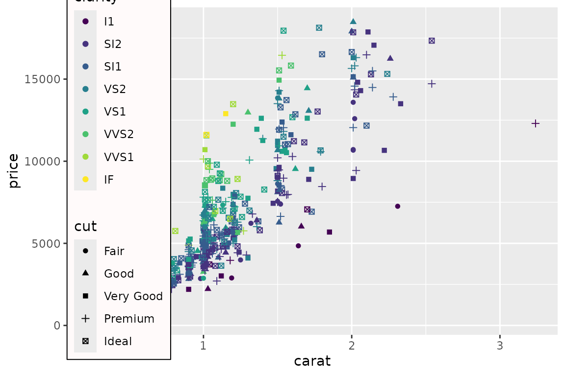

Legend with multple guides on a tacky ‘snow’ background.

Legends are placed under axis lines

The guidebox uses a solid background (subject to the chosen theme), and prior to lemon version 0.3.1, the entire legend was placed as the top most element. In the examples above, this was not an issue. With axis lines drawn, this effectively overpainted some of the axis (same applies to the panel border).

The guidebox is therefore placed under the lowest axis line, if and only if z = Inf. To place as top most, specify a large z-index.

reposition_legend(d + theme_classic(), 'top left')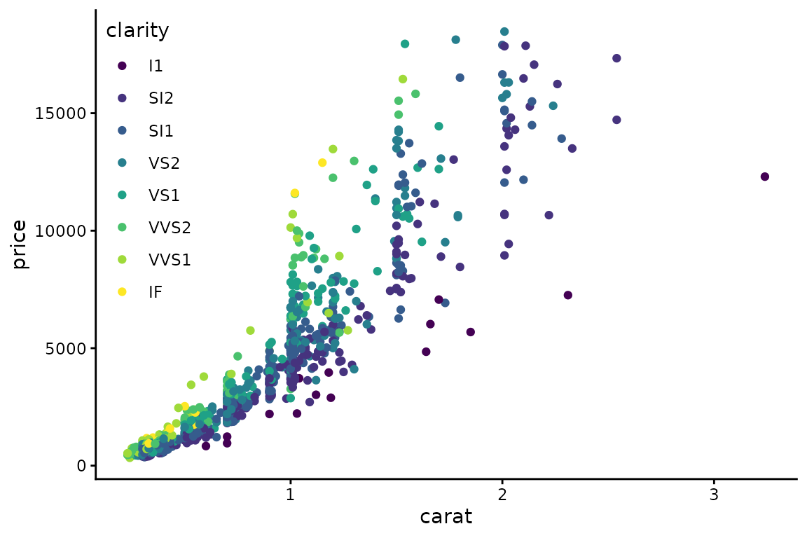

Legend is drawn under axis lines.

To adjust the guidebox so it does not overpaint the panel border, use arguments x and y,

reposition_legend(d + theme_bw(), 'top left', x=0.002, y=1-0.002)

Legend has to be nudged to not overpaint panel border.

… or use the argument offset:

reposition_legend(d + theme_bw(), 'top left', offset=0.002)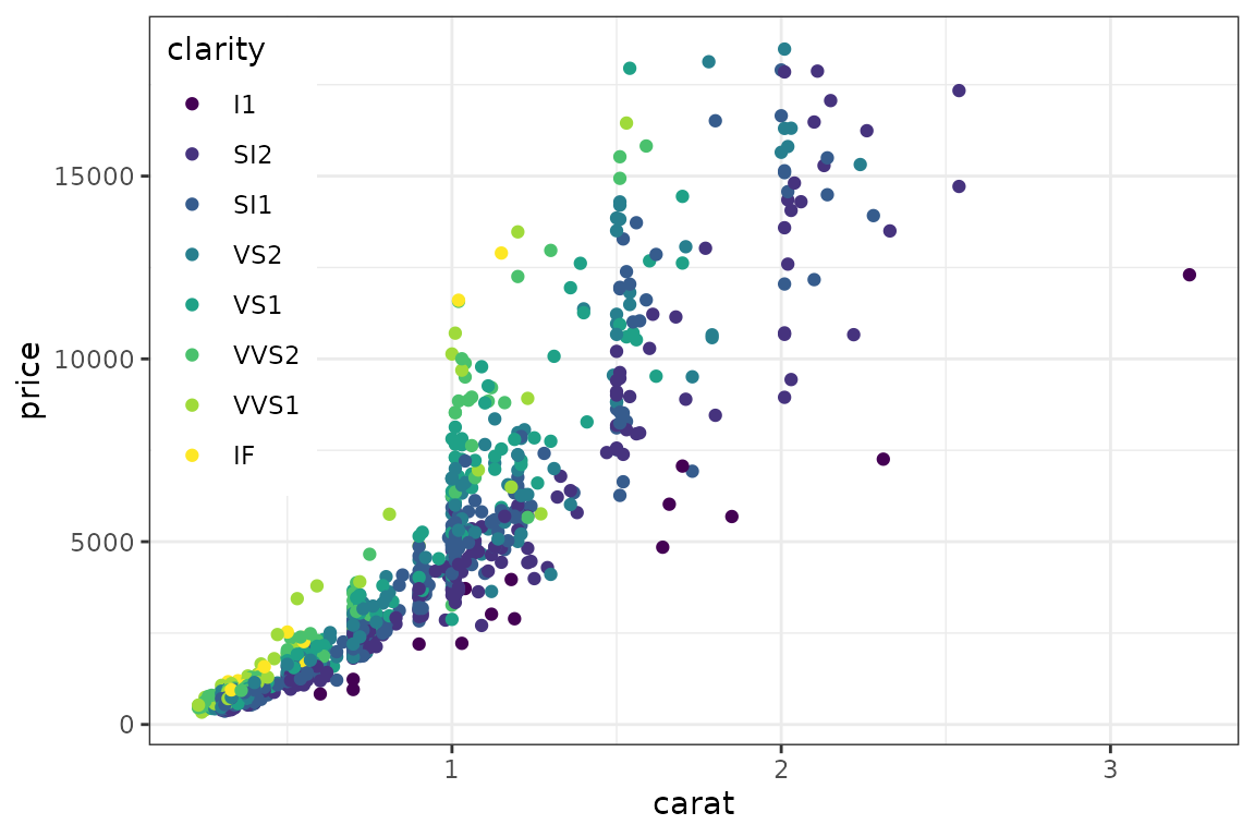

Legend has to be nudged to not overpaint panel border, this time by offset.

Warning regarding extracting legend

To our knowledge, there exists two methods for extracting the legend:

g1 <- function(a.gplot){
  if (!gtable::is.gtable(a.gplot))
    a.gplot <- ggplotGrob(a.gplot)
  leg <- which(sapply(a.gplot$grobs, function(x) x$name) == "guide-box")
  a.gplot$grobs[[leg]]
}
g2 <- function(a.gplot){
  if (!gtable::is.gtable(a.gplot))
    a.gplot <- ggplotGrob(a.gplot)
  gtable::gtable_filter(a.gplot, 'guide-box', fixed=TRUE)
}

There is very little difference between them, as the latter essentially does the same as the former. The latter however encapsulated the former in a gtable. This is even more evident with multiple guides:

(da <- ggplot(dsamp, aes(carat, price)) +
  geom_point(aes(colour = clarity, shape=cut)) +
   theme(legend.box = 'horizontal')
)

## Warning: Using shapes for an ordinal variable is not advised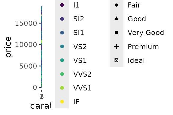

Two guides in a single legend, in a grossly undersized figure.

print(g1(da))

## Warning: Using shapes for an ordinal variable is not advised

## TableGrob (5 x 7) "guide-box": 3 grobs
##   z     cells                  name           grob
## 1 1 (3-3,3-3)                guides gtable[layout]
## 2 2 (3-3,5-5)                guides gtable[layout]
## 3 0 (2-4,2-6) legend.box.background zeroGrob[NULL]

print(g2(da))

## Warning: Using shapes for an ordinal variable is not advised

## TableGrob (9 x 9) "layout": 5 grobs
##    z     cells             name              grob
## 1 14 (5-5,9-9)  guide-box-right gtable[guide-box]
## 2 15 (5-5,1-1)   guide-box-left    zeroGrob[NULL]
## 3 16 (9-9,5-5) guide-box-bottom    zeroGrob[NULL]
## 4 17 (1-1,5-5)    guide-box-top    zeroGrob[NULL]
## 5 18 (5-5,5-5) guide-box-inside    zeroGrob[NULL]

The function reposition_legend assumes the method given in g1, which is also given in g_legend.

Placing the legend in facets

The above demonstration finds the panel named panel. This is default. If using facetting, the panels are typically named panel-{column}-{row}. We use gtable_show_names to display the names of the facetted panels.

d2 <- d + facet_grid(.~cut, )
gtable_show_names(d2)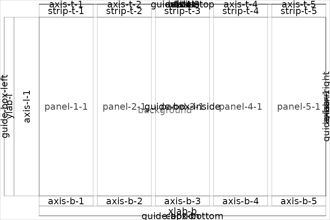

Facetted panels’ names.

So to place the legend in a specific panel, give its name. Depending on ggplot2 version, the panel’s name may differ.

try(reposition_legend(d2, 'top left', panel = 'panel-5-1'))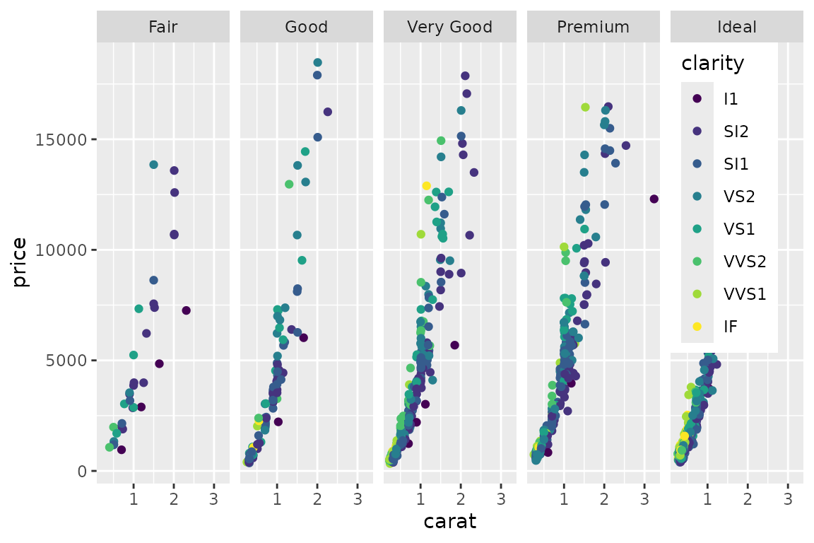

Placing the legend in a facet panel.

try(reposition_legend(d2, 'top left', panel = 'panel-1-5'))

## Error in reposition_legend(d2, "top left", panel = "panel-1-5") : 
##   Could not find panel named `panel-1-5`.

Likewise for facet_wrap. Incidentally, empty panels are also named here:

reposition_legend(d + facet_wrap(~cut, ncol=3), 'top left', panel='panel-3-2')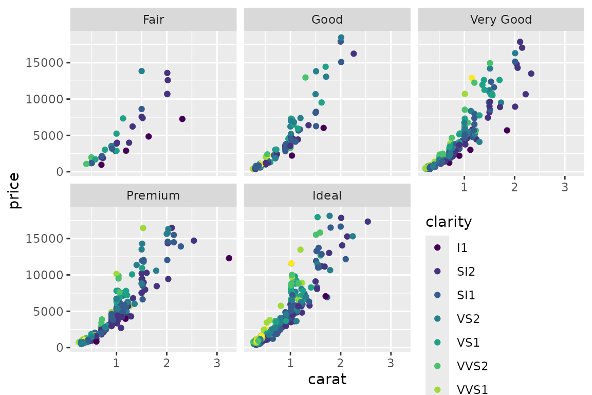

Placing the legend in an empty panel when using facet_wrap.

Modifying the legend is done via usual routines of ggplot2:

d3 <- d + facet_wrap(~cut, ncol=3) + scale_color_discrete(guide=guide_legend(ncol=3))
reposition_legend(d3, 'center', panel='panel-3-2')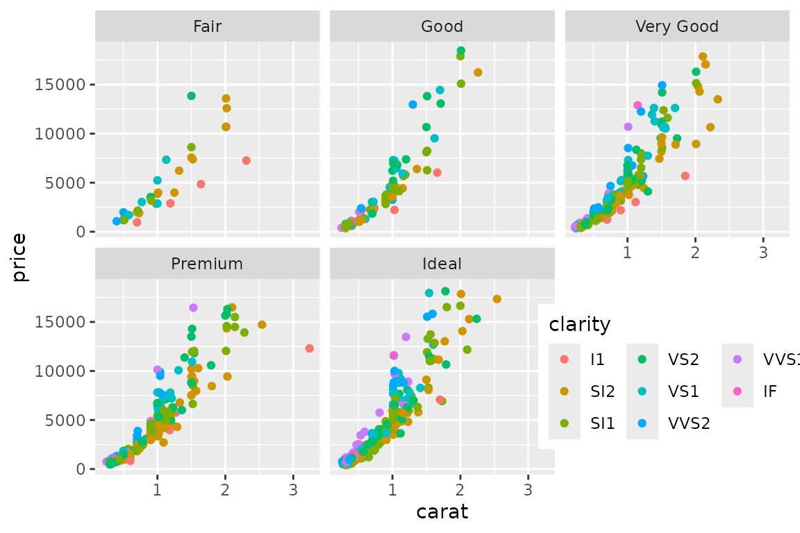

The looks of the legend is modified with usual ggplot2 options.

Also supports spanning multiple panels:

d4 <- d + facet_wrap(~cut, ncol=4) + scale_color_discrete(guide=guide_legend(nrow=2))
reposition_legend(d4, 'center', panel=c('panel-2-2','panel-4-2'))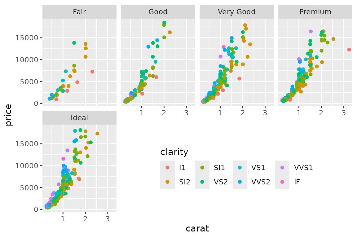

Supplying reposition_legend with multple panel-names allows the legend to span them.

The panel names are not easy to figure, especially those from facet_wrap. We refer to gtable_show_names to get a look at where they are:

gtable_show_names(d4)

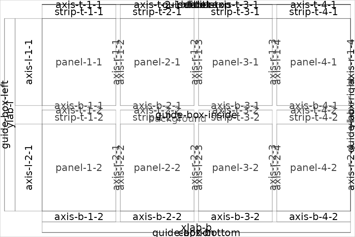
Use of gtable_show_names to reveal the panels’ names.

Shared legend across multiple plot

The function grid_arrange_shared_legend extracts the legend from its first argument, combines the plots with the legend hidden using arrangeGrob, and finally appends the legend to one of the sides. It even updates the plot’s theme to orientate the legend correctly.

dsamp <- diamonds[sample(nrow(diamonds), 1000), ]
p1 <- qplot(carat, price, data = dsamp, colour = clarity)

## Warning: `qplot()` was deprecated in ggplot2 3.4.0.
## This warning is displayed once every 8 hours.
## Call `lifecycle::last_lifecycle_warnings()` to see where this warning was
## generated.

p2 <- qplot(cut, price, data = dsamp, colour = clarity)
p3 <- qplot(color, price, data = dsamp, colour = clarity)
p4 <- qplot(depth, price, data = dsamp, colour = clarity)
grid_arrange_shared_legend(p1, p2, p3, p4, ncol = 2, nrow = 2, position='top')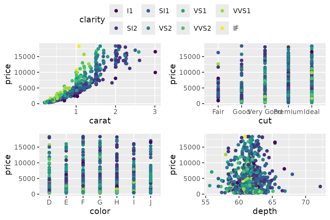

…

grid_arrange_shared_legend(p1, p2, p3, p4, ncol = 2, nrow = 2, position='bottom')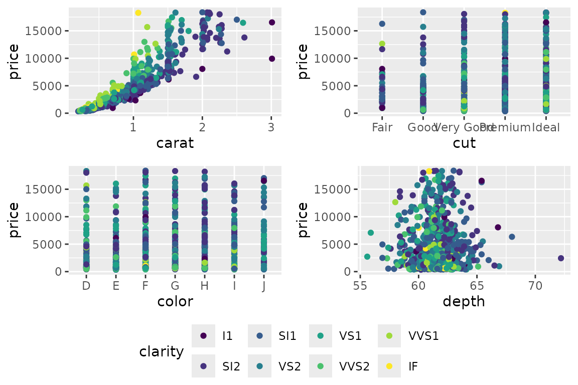

…

grid_arrange_shared_legend(p1, p2, p3, p4, ncol = 2, nrow = 2, position='left')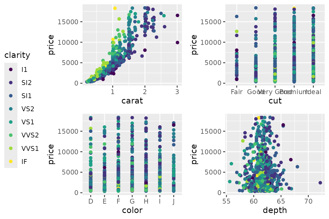

…

grid_arrange_shared_legend(p1, p2, p3, p4, ncol = 2, nrow = 2, position='right')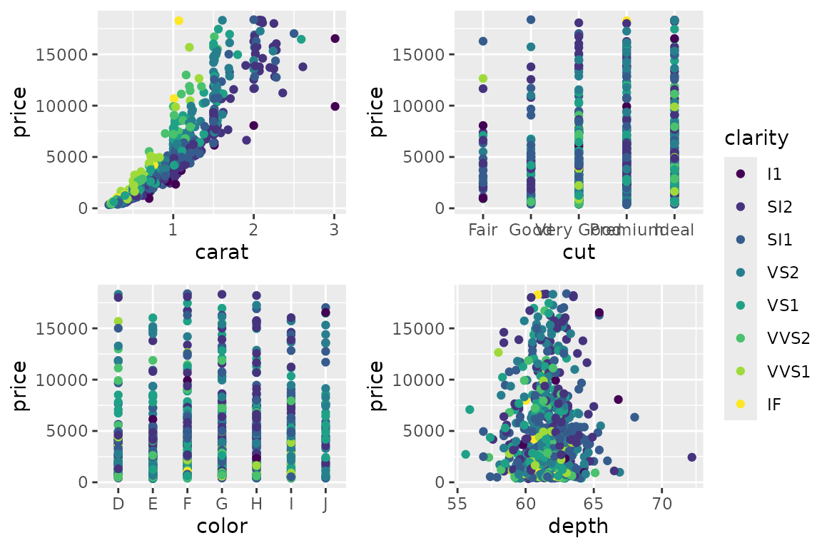

…

Shared legend with grid.arrange

A more flexible approach to combining plots and legends can be found in Baptiste Auguie’s gridExtra::grid.arrange and arrangeGrob. The latter is the power house that produces a grob object, which the former then draws to the device. But being more flexible, it is somewhat less automated.

We demonstrate here how to combine 3 of the 4 plots above, with different options for layout and placing the legend.

library(gridExtra)
legend <- g_legend(p1 + theme(legend.position='bottom'))
grid.arrange(p1+theme(legend.position='hidden'), p2+theme(legend.position='hidden'),
             p3+theme(legend.position='hidden'), legend)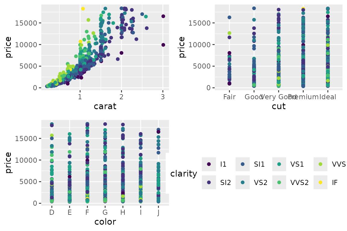

grid.arrange(p1+theme(legend.position='hidden'), p2+theme(legend.position='hidden'),
             p3+theme(legend.position='hidden'), legend,
             layout_matrix=matrix(c(1,3,4,2,3,4), ncol=2))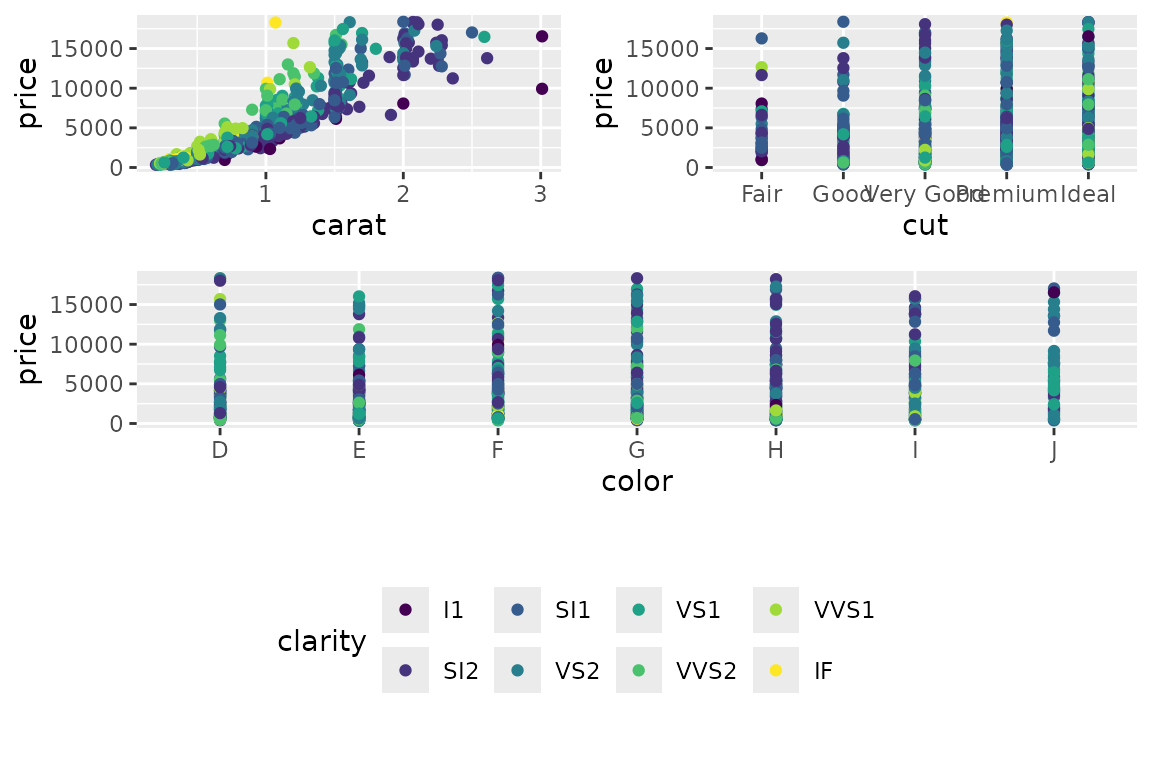

Using layout_matrix to have plots span different cells of a grid.

In the figure above, a layout matrix was defined with three rows. Subsequently, the three rows were of equal heights.

It is difficult to calculate the row heights to provide grid.arrange if we wanted to fix the height of the legend row’s height. We could attempt

(unit(1, 'npc') - sum(legend$heights)) / 2

but division is not permitted on units.

When grid.arrange is given a margin argument (e.g. bottom), it creates a gtable object with a row or column of appropiate dimension. The remainder of the gtable is re-sized to fit. We can therefore do:

grid.arrange(p1+theme(legend.position='hidden'), p2+theme(legend.position='hidden'),
             p3+theme(legend.position='hidden'), bottom=legend$grobs[[1]],
             layout_matrix=matrix(c(1,3,2,3), ncol=2))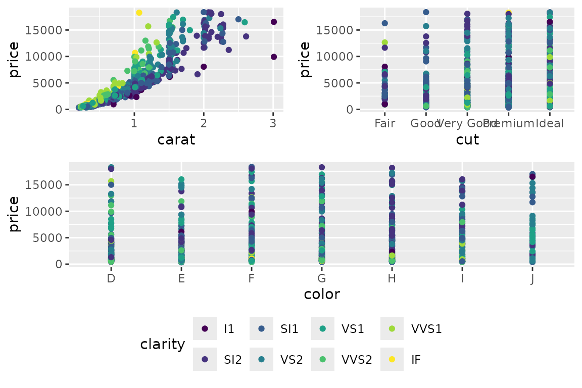

Using layout_matrix to have plots span different cells of a grid, but with legend in a separate argument.

There is however currently a shortcoming in grid.arrange and arrangeGrob that prevents it from using the full gtable object returned from g_legend in the margin arguments. We therefore subset to a specific grob.

What worse is, if the legend contains multiple guides, the above approach will not work directly. However, defining several arrangeGrob within each other is possible.

More examples

Complex layout with grid_arrange_shared_legend

Asked on: https://stackoverflow.com/questions/46238676/common-legend-for-a-grid-plot

In this reproducible example grid plot, 3 plots have 3 fill colours, and z displays with the “col” blue, but in the fourth plot there is only 1 “col”, so z displays as red.

I want to show only one common legend (which I can do), but I want z to be blue in all four plots. Is there a simple way to do that?

Before:

library(ggplot2)
library(grid)
library(gridExtra)

d0 <- read.csv(text="x, y, col\na,2,x\nb,2,y\nc,1,z")
d1 <- read.csv(text="x, y, col\na,2,x\nb,2,y\nc,1,z")
d2 <- read.csv(text="x, y, col\na,2,x\nb,2,y\nc,1,z")
d3 <- read.csv(text="x, y, col\na,2,z\nb,2,z\nc,1,z")
p0 <- ggplot(d0) + geom_col(mapping = aes(x, y, fill = col))
p1 <- ggplot(d1) + geom_col(mapping = aes(x, y, fill = col))
p2 <- ggplot(d2) + geom_col(mapping = aes(x, y, fill = col))
p3 <- ggplot(d3) + geom_col(mapping = aes(x, y, fill = col))
grid.arrange(p0, arrangeGrob(p1,p2,p3, ncol=3), ncol=1)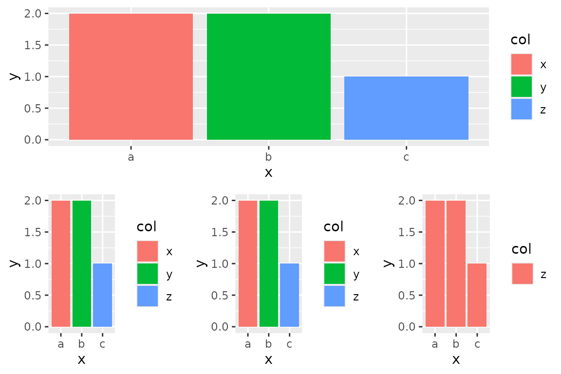

nt <- theme(legend.position='hidden')
grid_arrange_shared_legend(p0, arrangeGrob(p1+nt,p2+nt,p3+nt, ncol=3), ncol=1, nrow=2)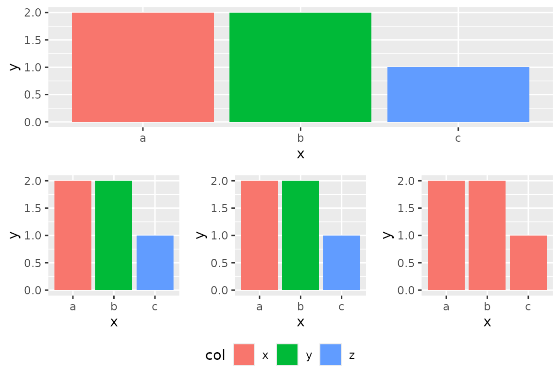

Plot for ggplot2-extensions

p <- ggplot(dsamp, aes(x=cut, y=price, colour=clarity)) + geom_point(position=position_jitter(width=0.2)) +
  coord_flex_cart(bottom=brackets_horizontal(), left=capped_vertical('none')) +
  theme_bw() + theme(panel.border=element_blank(), axis.line = element_line(),
                     legend.background = element_rect(colour='grey'))
g <- reposition_legend(p, 'top left', plot=TRUE)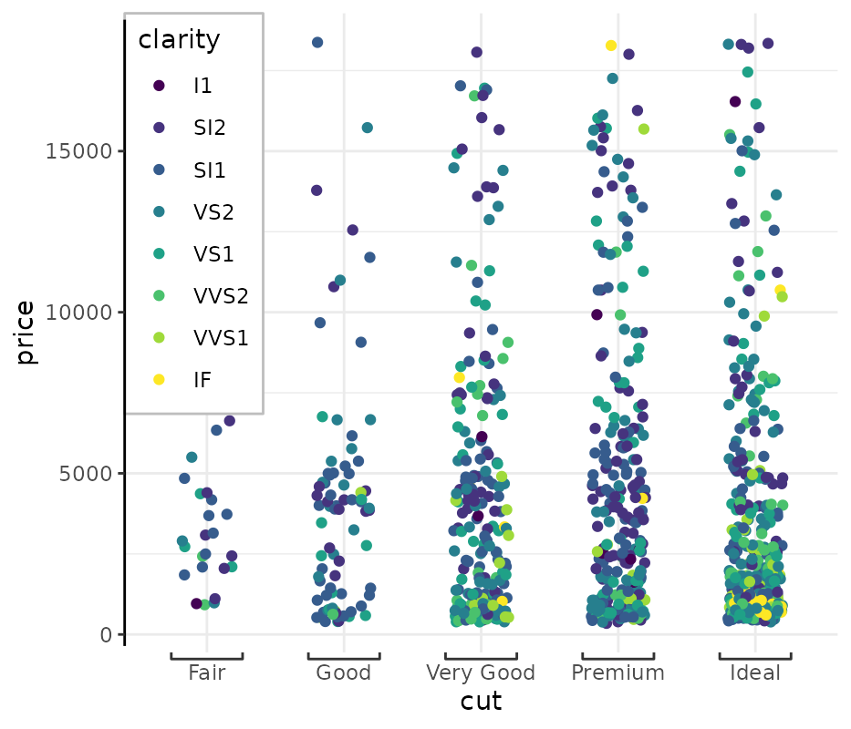

Acknowledgements

g_legend was proposed as early as June 2012 by Baptiste Auguié (http://baptiste.github.io/) on ggplot2’s wiki. It has since propogated throughout Stack Overflow answers.

Originally brought to you by (Baptiste Auguié)[http://baptiste.github.io/] (https://github.com/tidyverse/ggplot2/wiki/Share-a-legend-between-two-ggplot2-graphs) and (Shaun Jackman)[http://rpubs.com/sjackman] (http://rpubs.com/sjackman/grid_arrange_shared_legend). It has been further modified here.

reposition_legend was coded by Stefan McKinnon Edwards/

Footnotes

Example with reposition_legend that didn’t quite work:

dsamp <- diamonds[sample(nrow(diamonds), 1000), ]
d <- ggplot(dsamp, aes(carat, price)) +
  geom_point(aes(colour = clarity)) 
reposition_legend(d + theme_gray(base_size=26), 'top left')